

Abstract
Background/Objective: This ecological study examined whether regional differences in pharmacy naloxone dispensing–mortality associations were consistently supported across longitudinal analyses of U.S. states during 2012–2023.
Methods: The panel covered 50 states and the District of Columbia, with 610 available mortality outcomes among 612 potential state-years. State and year fixed-effects models assessed within-state regional associations. Random-intercept and generalized estimating equation (GEE) models included dispensing × region interactions and year effects. Fixed-effects and mixed models used state-cluster CR2 inference. Socioeconomic status (SES), Naloxone Access Laws (NALs), and one-year lags were exploratory.
Results: Within-state regional intervals spanned zero (joint slope-equality p = 0.237). A separate common-slope estimate was 1.712 deaths per 100,000 per dispensing SD (95% CI −0.810 to 4.235). Allowing for correlation within states through CR2 raised the random intercept joint p value from < .001 to .269 with the coefficients unchanged. The GEE joint p value was .152 with an independence working correlation and .033 with AR(1). Intervals for the SES interaction and the NAL coefficient included zero, and only the lag from prior year mortality to current dispensing had an interval excluding zero.
Conclusions: Support for regional differences depended on how persistent state differences and correlation within states were handled, so these data do not give a consistent regional ranking. Curvature, negative fitted rates, and unmeasured confounding that changes over time further limit what these state aggregates can show.
Keywords: opioid overdose, naloxone, geographic heterogeneity, socioeconomic status, Naloxone Access Laws, public health policy
Introduction
The U.S. overdose epidemic changed substantially during this period. National vital statistics showed the age-adjusted overdose death rate involving synthetic opioids other than methadone rose from 1.0 to 11.4 per 100,000 between 2013 and 20191. Research also documented health care and productivity costs of prescription opioid misuse2 and declining employment, hours, and earnings in states more exposed to the 2010 OxyContin reformulation and subsequent illicit opioid market expansion3.
Research on pharmacy naloxone access examines dispensing and laws intended to expand access. Naloxone is an opioid antagonist used to reverse acute opioid toxicity. A randomized prehospital trial documented responses in suspected heroin overdose4. Naloxone Access Laws (NALs) authorize standing orders, third-party prescribing, and pharmacist dispensing without patient-specific prescriptions5. Studies of NAL provisions and prescription dispensing reported differing evidence across provisions and populations6,7. These policy associations differ from the regional dispensing–mortality question.
Because NAL adoption spread while dispensing rose, an exploratory model relates adoption to dispensing after accounting for calendar year and region. With dispensing as its outcome, it describes the policy setting and does not estimate an NAL effect on mortality or mediation through dispensing.
Geographic variation in drug supply and services motivates regional dispensing–mortality comparisons. Pharmacy dispensing increased during 2012–2019 but differed substantially across states8. Forensic-test fentanyl exposure varied geographically and was associated with redistribution of all-drug overdose mortality during 2011–20179. Treatment programs in 2017 were unevenly distributed relative to opioid overdose deaths in 201610. The same dispensing rate could therefore occur alongside very different fentanyl exposure and treatment capacity, so the association between dispensing and mortality may differ by region.
U.S. studies have also linked opioid harm to socioeconomic conditions, associating unemployment with opioid analgesic mortality11 and multidimensional area deprivation with opioid mortality12, so the dispensing slope might differ with a state’s socioeconomic status. Education, income, and unemployment represent attainment, material resources, and employment conditions. The SES interaction is exploratory, with no assumed direction or inference about individual access mechanisms.
This study examined whether the association between pharmacy naloxone dispensing and opioid overdose mortality differed consistently across Census regions in annual state data from 2012 to 2023. Regional slopes were estimated with random intercept, generalized estimating equation (GEE), and state and year fixed effects models. All three include year effects. The random intercept model treats each state’s persistent mortality level as random and unrelated to dispensing, the fixed effects model removes that level, and the GEE models leave it in the residual and account for the resulting correlation through a working correlation and sandwich standard errors. Comparing them shows whether a regional difference comes from the slopes themselves or from the standard errors attached to them, and only a difference that holds in all three would justify explanations based on drug supply or treatment capacity.
Objectives
The primary objective was to compare regional slopes relating opioid overdose mortality to pharmacy naloxone dispensing and to assess whether their differences were consistent across longitudinal specifications. State and year fixed effects models were added during revision and take priority when the slopes are read as associations within states; a separate model with a single slope gives the pooled association. The analysis also describes state and regional trends and, through the ICC, how strongly observations cluster within states. Exploratory models ask whether the SES index modifies the dispensing slope, whether NAL adoption was associated with dispensing from 2012 to 2016, and whether each measure tracked the other’s value in the previous year. No ranking of regions was specified before analysis, so any ordering of the regional slopes is exploratory as well. All objectives are associational, because state aggregates observed over the same years cannot separate an effect of dispensing on mortality from dispensing that responds to overdose burden or from shared causes; the study therefore does not estimate the effectiveness of naloxone distribution or the direction of influence.
Methods
Data Sources
This observational panel covered all 50 U.S. states and the District of Columbia during 2012–2023, starting with Guy et al.’s Table 1 dispensing coverage in 20128. The exploratory NAL window was 2012–2016: jurisdictions coded 1 increased from 8 in 2012 to 48 in 2016. All 51 were coded 1 by 2017, eliminating same-year adopted–unadopted comparisons under this broad definition5.
Dispensing rates from two IQVIA Xponent sources covered retail, non-hospital pharmacy prescriptions with annual U.S. Census Bureau population denominators. Guy et al.’s Table 1 supplied 2012–2019 rates per 100,000, divided by 1,000 for rates per 100. The source reported approximately 92% coverage of prescriptions dispensed from community pharmacies without specifying geographic assignment8. CDC maps supplied 2020–2023 rates per 100 from projected new and refill retail prescriptions, covering nearly 94% of retail prescriptions and assigned by prescriber location. Mail-order and over-the-counter sales were excluded13. These measures count prescriptions, not doses administered, people treated, or overdose reversals, and omit non-pharmacy channels such as harm-reduction programs. Guy extraction and CDC download occurred December 28, 2025. All 612 exposures were available. Six Guy-reported zeros were retained, with no imputation.
Primary dispensing retained the December 28, 2025 acquisition version: 408 earlier rates matched Guy Table 1 after conversion. 204 later rates matched CDC data archived November 21, 2025. No exact download-day snapshot was available. A September 5, 2026 CDC snapshot differed in five 2023 values and was analyzed separately for source-version sensitivity.
KFF State Health Facts mortality exports, downloaded October 27, 2025, use National Vital Statistics System data through CDC WONDER. State opioid overdose death rates per 100,000 are age-adjusted to the 2000 U.S. standard population. Overdose ICD-10 underlying-cause codes were X40–X44, X60–X64, X85, or Y10–Y14. Opioid multiple-cause codes were T40.0, T40.1, T40.2, T40.3, T40.4, and T40.6. Illicitly manufactured and pharmaceutical fentanyl are included but not distinguished. NSD (not sufficient data), indicating fewer than 20 deaths, was treated as missing14. North Dakota’s unavailable 2012 and 2013 opioid rates were kept missing, without all-drug substitution. The source-export definition was retained without reconstructing an investigator-run WONDER query. Ten selected high- and low-burden jurisdiction rates exactly matched independent CDC/NCHS opioid-overdose rates.
Naloxone Access Law data came from the Prescription Drug Abuse Policy System (PDAPS), covering January 1, 2001–January 1, 2022 and downloaded November 9, 20255. Records coded 1 for the broad NAL item naaddressoaayn defined inclusive Effective Date–Valid Through Date intervals. Any calendar-year overlap was coded 1, otherwise 0, using effective rather than enactment dates without prorating partial years or delaying onset. Successive records were combined and provisions collapsed into one indicator. Record end dates were not treated as repeals, since a record can end when a law is amended, and no state moved from 1 back to 0 even where provisions changed. Reconstruction matched all 255 policy-model state-years.
The socioeconomic status (SES) index combined three American Community Survey (ACS) five year subject table estimates for endpoint years 2012 to 2023, which cover the periods from 2008 to 2012 through 2019 to 2023 and were downloaded on December 2, 2025. Education was the published percentage of the total population aged 25 years or older with a bachelor’s degree or higher (S1501)15, income was median household income in inflation adjusted dollars of each estimate’s endpoint year (S1901)16, and unemployment was the percentage of the civilian labor force aged 16 years or older that was unemployed (S2301)17. Each component was converted to a z score, and because higher unemployment indicates disadvantage, the unemployment z score was multiplied by −1 before the three z scores were averaged; the raw unemployment percentages were left unchanged. The average was standardized again to give the index. All of these means and sample SDs were computed over the 612 potential state years, before the two state years without mortality data were excluded.
Each signed, standardized component received one third of the weight, since no external source favored one domain and the weights were not fitted to the outcome. Because the components are correlated, their influence on the index can still differ after standardization, and the index is a descriptive summary that has not been validated as a latent SES measure.
States were assigned to the four U.S. Census Bureau regions (Northeast, Midwest, South, and West)18.
Variables
The primary outcome was the age adjusted opioid overdose death rate per 100,000, and the exposure was standardized dispensing. Region was categorical (Northeast reference unless noted), SES a secondary moderator, and NAL adoption a binary exploratory policy predictor.
Mortality is age-adjusted for age-structure comparisons. Dispensing uses a crude population denominator. Coefficients relate differently standardized measures, not age-specific effects. Dispensing cannot be age-standardized without age-specific prescription counts.
The exposure and SES terms used in interaction models were standardized. Mortality remained in deaths per 100,000:
(1) 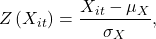
where μX and σX denote the sample mean and standard deviation of variable X, respectively. For the reference mixed model, both regional GEE models, and state/year fixed-effects models, dispensing used the pooled mean and sample SD of the same 610 complete state-years (mean 0.219369, SD 0.303618 prescriptions per 100). These values also standardized the refreshed-CDC sensitivity input. For the SES model, each component, the equal-weight composite, and dispensing were standardized over all 612 potential state-years before mortality exclusions. The forward-lag dispensing predictor and reverse-lag mortality predictor were standardized over their respective 560- and 559-observation samples. No variable was standardized separately by year, region, or state. Mortality outcomes and NAL-model dispensing outcomes remained in their original rate units.
Ethical Considerations
Only publicly available, aggregate, de-identified secondary data from federal agencies and a public policy surveillance system were used. No participants were contacted or identifiable private information accessed. Institutional review board approval and informed consent were therefore not required. State-level aggregation prevents identification of individuals in the reported results.
Statistical Analysis
Exploratory Data Analyses
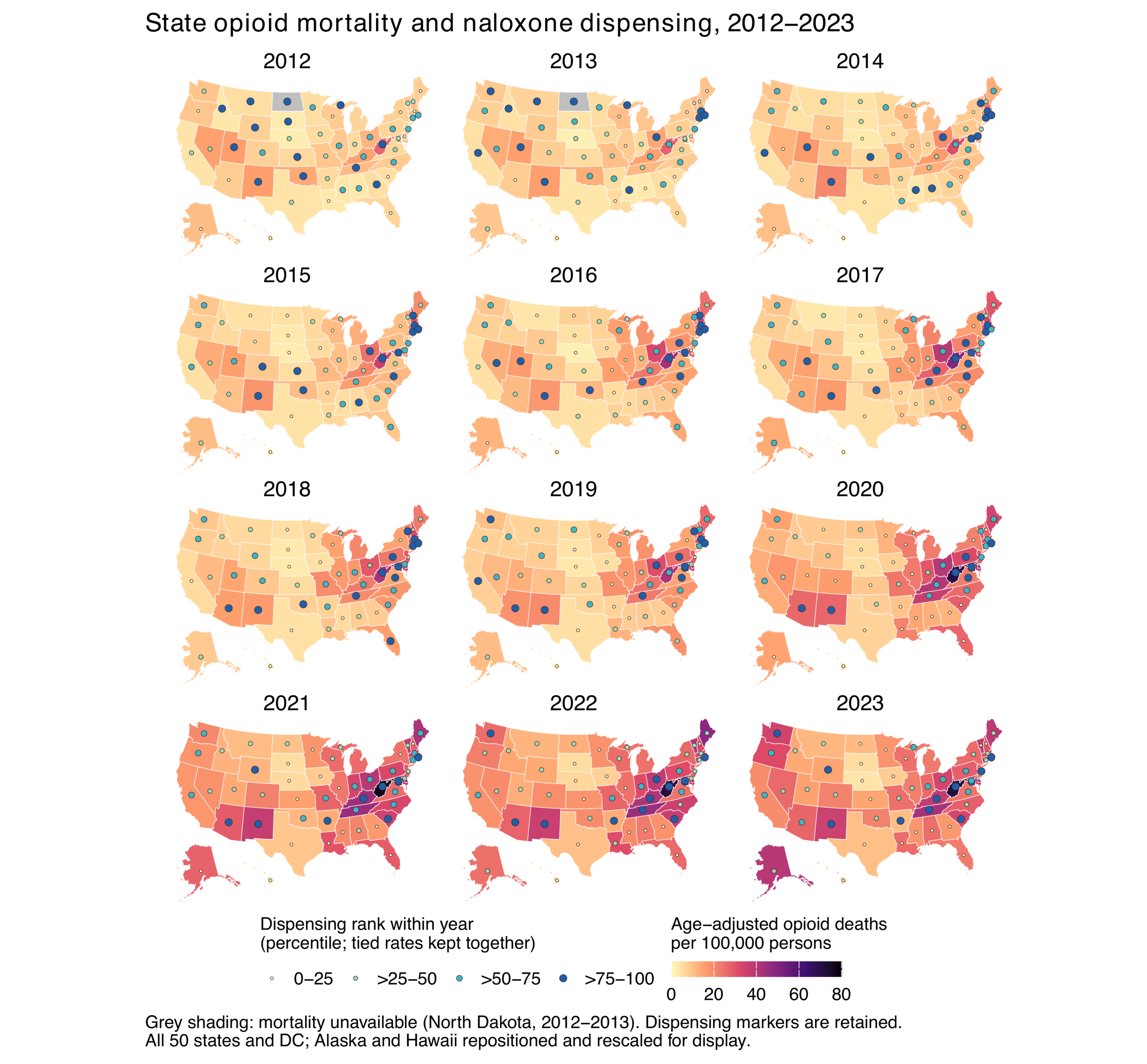
Annual maps showed mortality and within-year dispensing percentiles, assigning ties the same percentile. Regional and overall trends were unweighted means of available state/DC rates, not population-weighted national rates. Missing mortality was omitted from means and distinguished on maps. These displays describe co-occurrence without establishing causality.
Mixed-Effects Models
The reference random-intercept specification used standardized dispensing, Census region, their interaction, categorical year effects, and state intercepts, fitted by maximum likelihood to 610 complete state-years:
(2) 
Here, i indexes states and t indexes years. Deathit denotes the opioid overdose death rate, Dispit denotes standardized naloxone dispensing, Regioni denotes U.S. Census region, and γt represents year fixed effects. The state-level random intercept was specified as ui ∼ 𝒩(0, σu2), and the residual error term was specified as εit ∼ 𝒩(0, σ2).
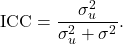
The intraclass correlation coefficient (ICC) describes state clustering’s share of residual variance, conditional on covariates and the specified random-intercept model:
(3) 
A secondary mixed-effects model examined whether SES moderated the dispensing–mortality association:
(4) 
The interaction term Dispit × SESit tested whether the association between naloxone dispensing and overdose mortality differed across state-level socioeconomic contexts.
An exploratory 2012–2016 policy model related NAL adoption to naloxone dispensing:
(5) 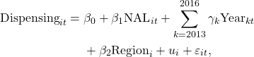
In this model, NALit was equal to 1 if any positive PDAPS interval overlapped the calendar year in state i during year t, and 0 otherwise. The model estimates an adjusted association with dispensing using categorical year and region terms and a state random intercept. Mortality is not its outcome.
Generalized Estimating Equation Models
The GEE models used a Gaussian family with an identity link and kept the sample, dispensing scale, dispensing × region interaction, and categorical year effects of the reference mixed model. With X denoting the included covariates, the conditional mean was:
(6) 
Two GEE models were fitted, one with an independence and one with a first order autoregressive, AR(1), working correlation, both using a sandwich covariance estimator clustered by state19 with observations ordered by state and actual calendar year. Because the mean is linear, averaging over a random intercept with mean zero given the covariates leaves the fixed slopes unchanged20, so the GEE and random intercept models target the same slopes. Their estimates and standard errors can still differ through the weighting implied by the working correlation or through violated mean, covariance, or exogeneity assumptions. The GEE results therefore measure the sensitivity of the regional comparison to these choices and do not count as independent confirmation.
Contrasts using the full coefficient covariance gave the four regional slopes, their six pairwise differences with pointwise intervals, and a joint test of equal slopes. Conventional Satterthwaite t and F tests for the mixed model (lmerTest21) were kept for comparison with CR2, GEE used normal and χ² Wald tests, and Holm’s procedure adjusted the six pairwise p values within each model and data version22. Region main effects give mortality levels at mean dispensing.
Within-State and Sensitivity Analyses
State and calendar year fixed effects models, fitted to the same 610 observations and dispensing scale, estimated either four regional slopes or one common slope, and state effects absorbed the region main effects because each state lies in one region. Removing each state’s persistent level and the changes shared by all states in a year gives these models priority for associations within states. Inference used CR2 standard errors clustered by state, Satterthwaite t intervals, and the small sample HTZ test of equal slopes23. The unchanged random-intercept fit used the same inference framework through clubSandwich’s lmerMod implementation24, separating uncertainty calculation from mean specification. The common-slope specification provides a separate pooled summary under a shared-slope assumption. Its test against zero does not test regional equality.
Temporal structure was summarized by unweighted annual means and dispensing variation explained by year and state plus year effects. Residual SD and range described remaining exposure variation.
Forward and reverse models related current mortality to preceding-calendar-year dispensing and current dispensing to preceding-calendar-year mortality, respectively (N = 560 and 559). Within-state lags preceded exclusions and never bridged calendar-year gaps. Both used region, categorical year effects, and state random intercepts. Temporal precedence neither eliminates confounding nor identifies causal direction.
All five mixed models underwent conditional residual-versus-fitted and quantile plots, scaled spread by year/region, consecutive-year residual correlations without bridging gaps, random-intercept quantile plots, and negative fitted-rate counts. Following diagnostics during revision, state-cluster CR2 SEs and Satterthwaite intervals became preferred for every mixed model, regardless of interval widening or narrowing. This was not prespecified. Coefficients and samples were unchanged. Model reports retain labeled model-based comparisons. CR2 used fitted-model working targets in clubSandwich 0.6.123,24. These inference changes apply to the corrected-data fits and are distinct from the mortality and education data corrections made during revision. Complete common- and regional-slope fixed-effects models were additionally checked using residual and quantile plots, spread and serial-dependence summaries, negative fitted counts, and leave-one-state-out slope changes. No diagnostic exclusions were adopted.
Analyses were run in R with lme4, lmerTest, geepack, clubSandwich, and modelsummary, and the original sources, corrected inputs, scripts, sample keys, covariance matrices, and full precision estimates were retained. Mixed-model R² followed Nakagawa and Schielzeth’s variance-partition framework25. Marginal R² divided sample variance of fixed-effect predictions (denominator n − 1) by its sum with state-intercept and residual variances. Conditional R² added state-intercept variance to the numerator.
| Variable | Mean | SD | Minimum | Maximum |
| Opioid overdose death rate per 100,000 | 17.102 | 11.846 | 2.200 | 77.200 |
| Naloxone dispensing rate per 100 population | 0.219 | 0.303 | 0.000 | 2.500 |
| Bachelor’s degree or higher (%) | 31.103 | 6.559 | 17.900 | 63.600 |
| Median household income (endpoint-year $) | 61,710 | 13,156 | 38,882 | 106,287 |
| Unemployment rate (%) | 6.436 | 2.074 | 2.700 | 12.700 |
| SES index (z-score) | 0.000 | 1.000 | -2.330 | 3.428 |
| NAL adoption indicator | 0.569 | 0.496 | 0.000 | 1.000 |
Available observations: mortality N = 610, dispensing, SES components, and SES index N = 612. NAL covers 2012–2016 (N = 255). Income uses ACS endpoint-year dollars without common-price-year conversion. Each observation is one state in one year. Reported dispensing zeros were retained, and the sample for each model is reported with that model.
Results
Table 1 summarizes the data. All results use the dispensing values that matched Guy et al.’s Table 1 and the archived CDC data, together with the corrected mortality outcomes, and the fixed effects analysis within states is reported before the random intercept and GEE comparisons.
Exploratory Data Analysis
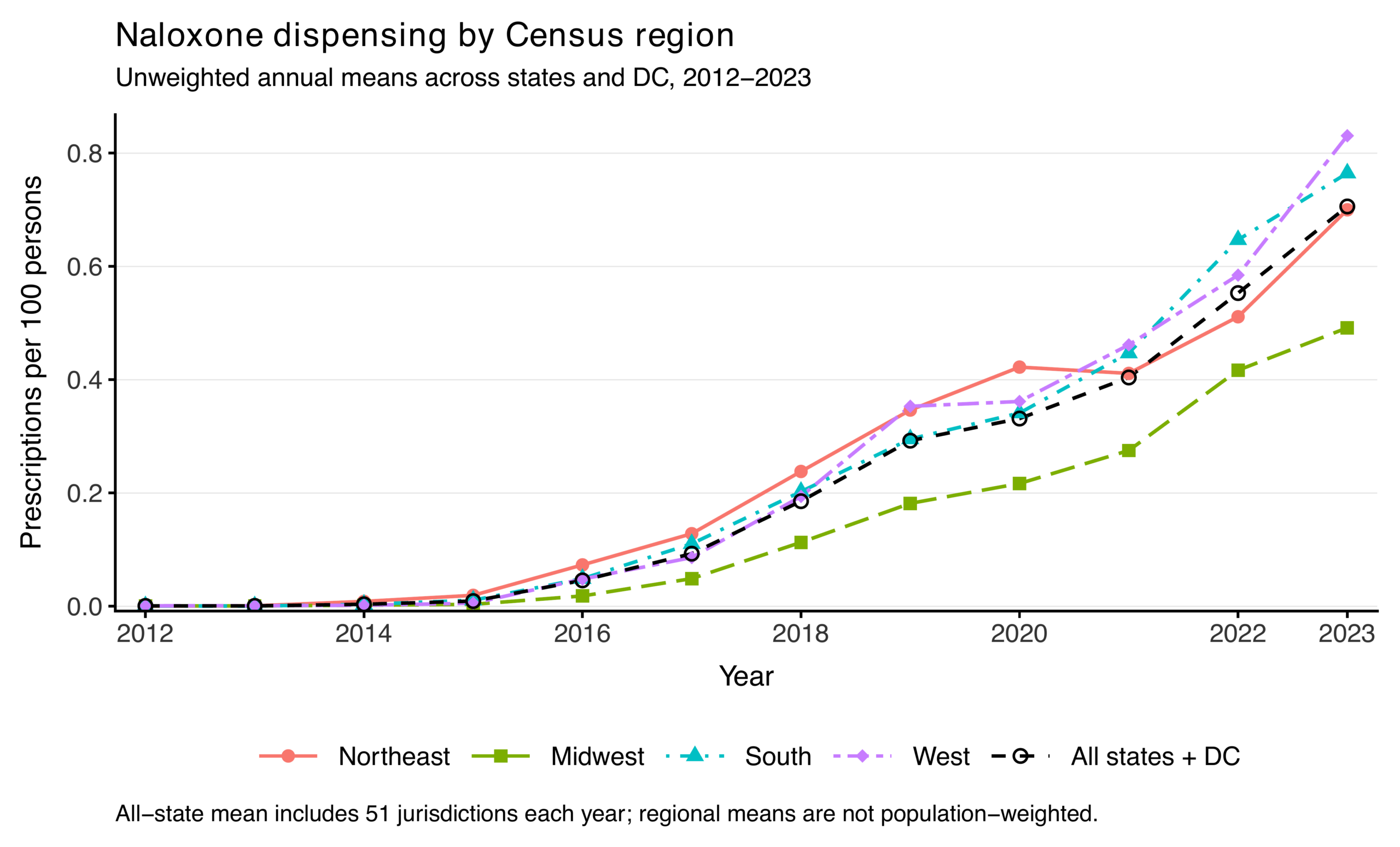
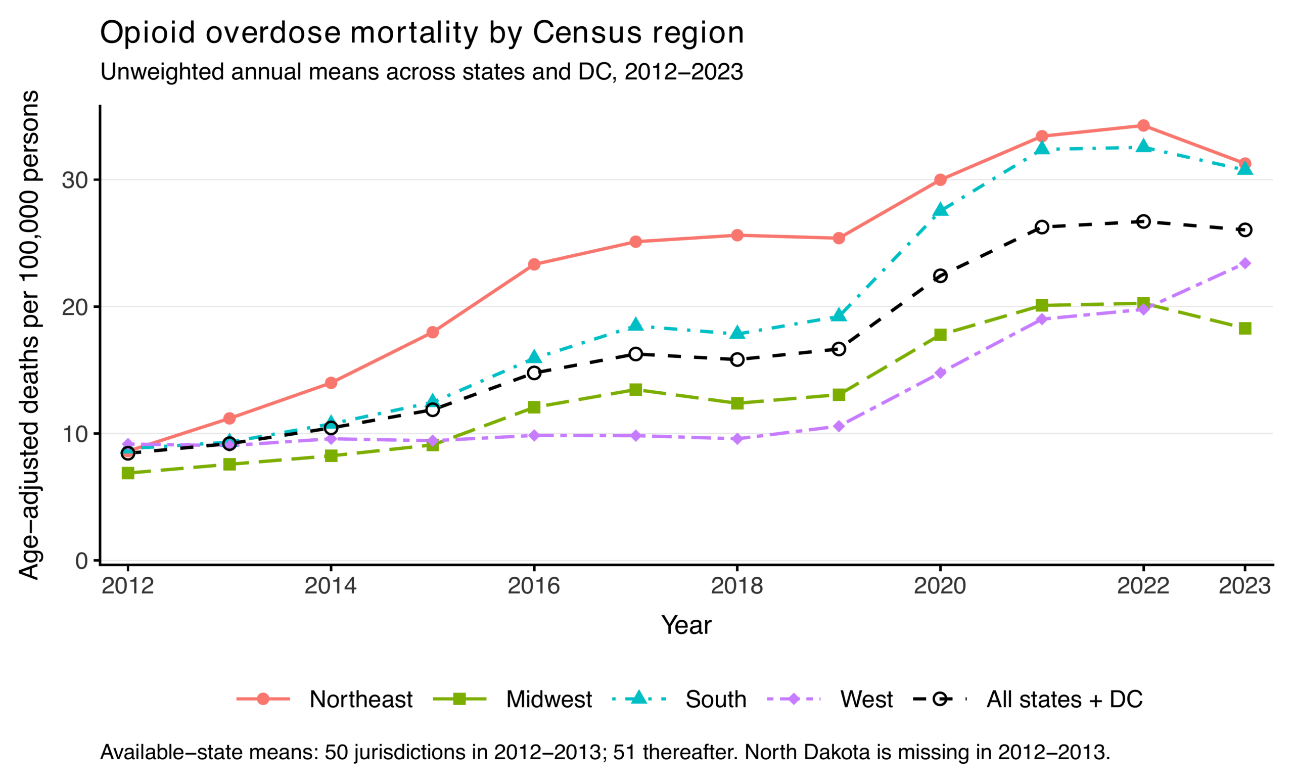
Mortality and pharmacy dispensing varied widely across states and years (Figure 1). Because the two measures are in different units, Figures 2 and 3 plot their regional and overall means separately.
Unweighted mean dispensing across the states and DC rose in each of the 11 annual intervals, although only 13 of the 51 state series never declined. Unweighted mean mortality rose by 17.601 deaths per 100,000, from 8.442 in 2012 to 26.043 in 2023, with nine annual increases and two decreases; the 2012 and 2013 means use 50 jurisdictions because North Dakota’s mortality is missing.
Within-State Dispensing–Mortality Associations
In the state and year fixed effects model, the 95% intervals for all four regional slopes included zero (Table 2), and the test of equal slopes gave F(3, 10.96) = 1.641, p = .237. A separate model imposing a common slope gave an estimate of 1.712 deaths per 100,000 per dispensing SD (95% CI −0.810 to 4.235, p = .158). In the same 610-observation sample, year effects explained 57.4% of dispensing variation and state plus year effects explained 72.3%. Residual dispensing had SD 0.160 per 100 (range −0.444 to 1.610), compared with the unadjusted SD of 0.304.
| Specification / region | Estimate [95% CI] | df | p |
| Common slope | 1.712 [-0.810, 4.235] | 8.56 | 0.158 |
| Northeast | 1.969 [-2.395, 6.333] | 4.82 | 0.295 |
| Midwest | -0.198 [-4.076, 3.680] | 11.34 | 0.913 |
| South | 3.073 [-1.545, 7.691] | 7.44 | 0.161 |
| West | 0.089 [-2.417, 2.595] | 3.24 | 0.920 |
Common and regional slopes use separate specifications, each with 610 state-years and 51 state/DC clusters. Units are deaths per 100,000 per primary-sample SD higher dispensing. State-cluster CR2 SEs yield pointwise 95% Satterthwaite t intervals with coefficient-specific effective degrees of freedom. The joint regional test uses HTZ.
Geographic Heterogeneity in the Dispensing–Mortality Association
In the reference random-intercept fit, regional slopes per one reference-sample SD higher dispensing were 2.099 in the Northeast (95% CR2 CI −2.328 to 6.527), 0.117 in the Midwest (−3.797 to 4.030), 3.226 in the South (−1.530 to 7.982), and 0.224 in the West (−2.424 to 2.871), so every interval again included zero (Table 3, Figure 4).
| RI: Death ∼ Dispensing × Region | |
| Intercept | 15.623 (1.551) [12.120, 19.126] |
| Naloxone dispensing (z-score) | 2.099 (1.698) [-2.328, 6.527] |
| Region: Midwest (vs Northeast) | -10.033 (2.677) [-15.668, -4.398] |
| Region: South (vs Northeast) | -3.759 (2.742) [-9.560, 2.042] |
| Region: West (vs Northeast) | -10.396 (1.772) [-14.128, -6.665] |
| Dispensing × Midwest | -1.982 (1.720) [-5.738, 1.773] |
| Dispensing × South | 1.126 (1.986) [-3.654, 5.907] |
| Dispensing × West | -1.875 (1.504) [-5.511, 1.760] |
| Year 2013 (vs 2012) | 0.758 (0.225) [0.306, 1.210] |
| Year 2014 (vs 2012) | 2.161 (0.414) [1.330, 2.993] |
| Year 2015 (vs 2012) | 3.555 (0.651) [2.247, 4.862] |
| Year 2016 (vs 2012) | 6.245 (0.978) [4.281, 8.209] |
| Year 2017 (vs 2012) | 7.442 (1.197) [5.038, 9.846] |
| Year 2018 (vs 2012) | 6.516 (1.370) [3.762, 9.270] |
| Year 2019 (vs 2012) | 6.852 (1.638) [3.556, 10.148] |
| Year 2020 (vs 2012) | 12.359 (1.882) [8.571, 16.147] |
| Year 2021 (vs 2012) | 15.815 (2.104) [11.579, 20.051] |
| Year 2022 (vs 2012) | 15.388 (2.434) [10.467, 20.309] |
| Year 2023 (vs 2012) | 14.027 (2.824) [8.315, 19.739] |
| Observations | 610 |
| Marginal R2 | 0.456 |
| Conditional R2 | 0.838 |
| ICC (state-level random intercept) | 0.702 |
Maximum-likelihood state random-intercept fit with year effects. Northeast and 2012 are references. Cells give the estimate, CR2 SE (in parentheses), and pointwise 95% Satterthwaite t interval [in brackets], with dispensing standardized over 610 state years. CR2 replaced conventional SEs after the diagnostics; conventional results are kept for comparison in the model reports
The estimated ICC was 0.702, so in the fitted random intercept model the state intercepts accounted for about 70% of the residual variance left after the covariates. Adding the state intercepts raised the share of variance explained from 0.456 (marginal R²) to 0.838 (conditional R²).
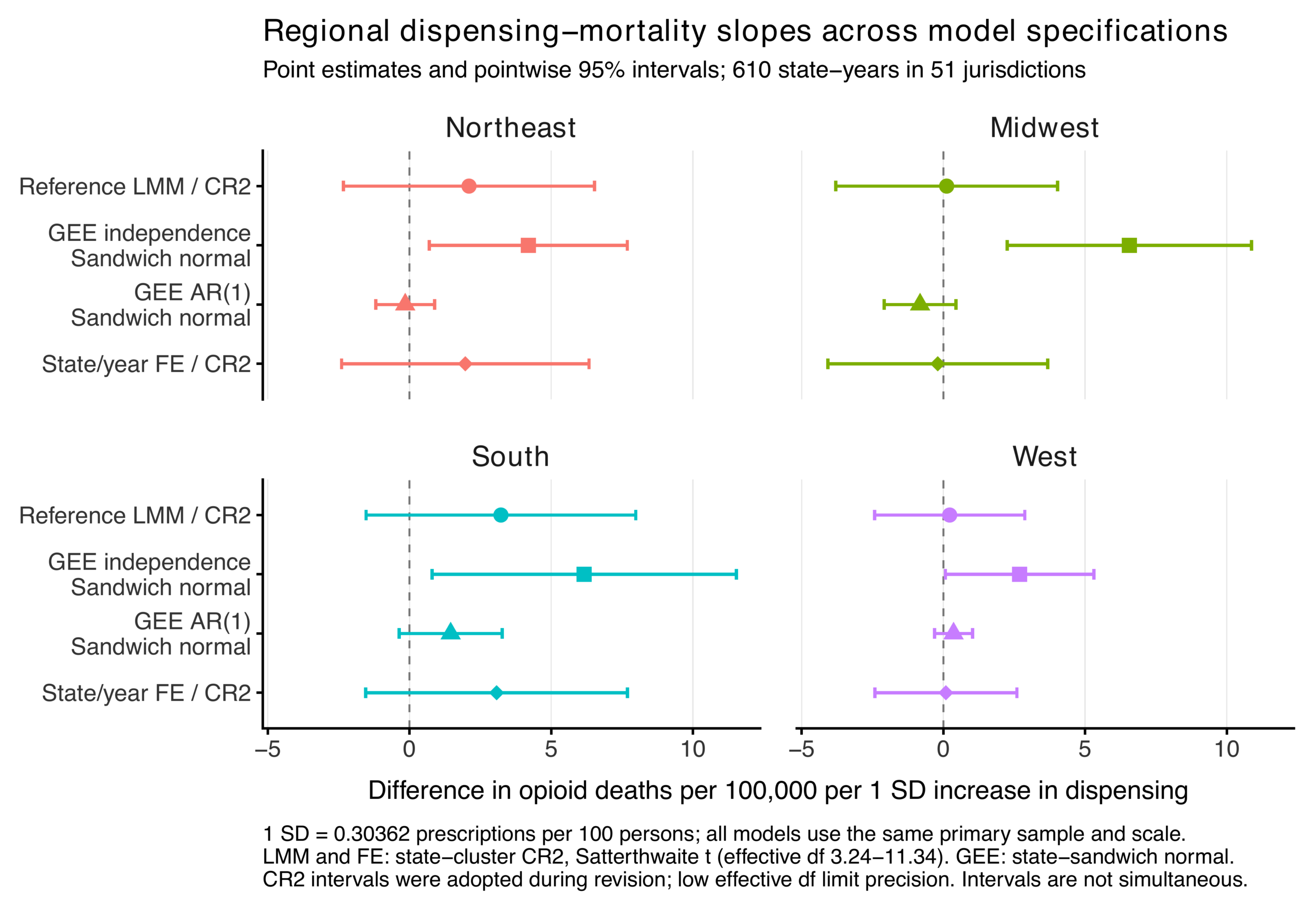
The CR2 joint test for the random intercept model gave F(3, 10.94) = 1.501, p = .269, and no Holm adjusted pairwise p value fell below .566; the South and Northeast contrast, for example, was 1.126 (95% CR2 CI −3.654 to 5.907, unadjusted p = 0.590, Holm p = 1.000), so the regions cannot be ranked. The conventional joint p < .001 for the same coefficients is reported only to compare covariance estimators.
Table 3 year coefficients describe conditional mortality differences relative to 2012.
Population-Averaged GEE Models
Table 4 reports GEE regional slopes using the mixed model’s dispensing × region interaction.
Under independence GEE, all four slope intervals excluded zero, but the joint slope-equality test yielded χ²(3) = 5.287, p = .152. Under AR(1), with an estimated working correlation of 0.914, all four individual intervals included zero, yet the joint test gave χ²(3) = 8.766, p = .033.
| Region / statistic | GEE independence | GEE AR(1) |
| Northeast | 4.193 [0.700, 7.685] | -0.151 [-1.190, 0.888] |
| Midwest | 6.564 [2.254, 10.875] | -0.821 [-2.087, 0.445] |
| South | 6.163 [0.795, 11.530] | 1.453 [-0.365, 3.271] |
| West | 2.690 [0.072, 5.309] | 0.361 [-0.312, 1.033] |
| Joint regional p | .152 | .033 |
| Year fixed effects | Included | Included |
| Observations / states | 610 / 51 | 610 / 51 |
Slopes [pointwise 95% CI] are deaths per 100,000 per primary-sample SD higher dispensing. Both models include year effects, N = 610, and 51 state/DC clusters. Robust state-sandwich normal inference is asymptotic over clusters. The joint p value tests equality of four slopes, not individual slopes against zero.
No independence-GEE pairwise contrast met the .05 threshold after Holm adjustment. Under AR(1), the Midwest–South difference was −2.274 (95% CI −3.904 to −0.644, unadjusted p = .00625, Holm p = .0375). Individual slopes and differences between correlated slopes test distinct hypotheses. The regional pattern was not consistent across the two working correlations.
Exploratory Analyses
With CR2 inference, the SES-model dispensing estimate at mean SES was 1.766 (95% CI −0.919 to 4.450, p = .164), and the SES estimate at mean dispensing was 3.713 (−1.686 to 9.113, p = .171). The interaction was 0.114 (−1.923 to 2.150, p = .896, 6.15 effective degrees of freedom). All intervals included zero (Table 5).
| RI: Death ∼ Dispensing × SES | |
| Intercept | 12.647 (1.772) [9.061, 16.233] |
| Naloxone dispensing (z-score) | 1.766 (1.134) [-0.919, 4.450] |
| SES index (z-score) | 3.713 (2.646) [-1.686, 9.113] |
| Dispensing × SES | 0.114 (0.837) [-1.923, 2.150] |
| Year fixed effects | Included |
| Observations | 610 |
| Marginal R2 | 0.341 |
| Conditional R2 | 0.845 |
| ICC (state-level random intercept) | 0.765 |
State random-intercept fit with year effects (2012 reference). Cells give estimate (CR2 SE) and pointwise 95% Satterthwaite t interval. Dispensing and SES use pooled standardization over 612 potential state-years before two unavailable outcomes are excluded. Each main coefficient is evaluated at the other variable’s mean. Model-based inference is retained separately for comparison.
The SES model used 610 observations after standardization over 612 potential state-years. Marginal R² was 0.341, conditional R² was 0.845, and the model residual ICC was 0.765.
The exploratory NAL model related adoption to dispensing during 2012–2016 (N = 255 state-years).
The NAL coefficient was −0.0030 prescriptions per 100 population (95% CR2 CI −0.0080 to 0.0020, p = .227, 40.99 effective degrees of freedom). The dispensing-model ICC was .118. Midwest and 2012 were references.
Lagged Sensitivity Analyses
Table 6 reports one-year lagged associations using corrected mortality and exact preceding-calendar-year values.
Prior-year standardized dispensing had a positive point estimate for current mortality: 2.139 deaths per 100,000 (95% CR2 CI −0.033 to 4.311, p = .0528, 8.34 effective degrees of freedom, N = 560). Its model-based interval, 1.395 to 2.883, illustrates sensitivity to uncertainty calculation. The preferred interval included zero.
| Deatht ∼Dispensingt − 1 | Dispensingt ∼Deatht − 1 | |
| Intercept | 17.172 (1.484) [13.813, 20.532] | 0.031 (0.038) [-0.051, 0.113] |
| Lagged naloxone dispensing (z-score) | 2.139 (0.949) [-0.033, 4.311] | — |
| Lagged overdose death (z-score) | — | 0.075 (0.027) [0.019, 0.131] |
| Region: Midwest (vs Northeast) | -10.205 (2.551) [-15.576, -4.834] | -0.036 (0.048) [-0.136, 0.064] |
| Region: South (vs Northeast) | -3.988 (2.979) [-10.291, 2.314] | 0.027 (0.051) [-0.081, 0.135] |
| Region: West (vs Northeast) | -11.466 (1.722) [-15.093, -7.839] | 0.076 (0.062) [-0.052, 0.205] |
| Year fixed effects | Included | Included |
| Observations | 560 | 559 |
| Marginal R2 | 0.437 | 0.611 |
| Conditional R2 | 0.842 | 0.703 |
State random-intercept fits include region (Northeast reference) and year effects (2013 reference). Cells give the estimate, CR2 SE (in parentheses), and pointwise 95% Satterthwaite t interval [in brackets]. The forward lag outcome is mortality (deaths per 100,000) and the reverse lag outcome is dispensing (prescriptions per 100), so R² is not comparable between them; each lagged predictor is standardized within its own model sample.
In the reverse direction, each SD of higher prior year mortality was associated with 0.075 more prescriptions per 100 (95% CR2 CI 0.019 to 0.131, p = .0120, 17.30 effective degrees of freedom, N = 559), and unlike the forward lag interval, this one excluded zero.
Source-Version Sensitivity and Model Diagnostics
Substituting the five 2023 dispensing values that differed in the September 2026 CDC snapshot, with sample and standardization fixed, changed no regional slope in the mixed model or either GEE by more than 0.0366 deaths per 100,000 per SD, reversed no sign or Holm adjusted pairwise decision at .05, and moved the fixed effects joint p value from .237 to .235.
Residual plots showed curvature, spread that changed with fitted value and year, and departures in the quantile tails, most clearly when dispensing was the outcome. Correlations between a state’s residuals in consecutive years were .760, .774, .728, .591, and .378 in the regional, SES, forward lag, reverse lag, and NAL models. Every mixed model produced some negative conditional fitted rates, reaching 20.8% (116 of 559) in the reverse lag model and 29.0% (74 of 255) in the NAL model. The common- and regional-slope fixed-effects models likewise showed curvature, unequal spread and tail departures, with consecutive-year residual correlations of .779 and .760 and negative fitted rates in 20/610 (3.3%) and 19/610 (3.1%) observations.
Discussion
The analyses did not establish a consistent regional pattern in dispensing–mortality associations. Within-state estimates were imprecise (joint slope-equality p = .237) but remained close to the random-intercept estimates: Northeast slopes were 1.969 and 2.099, respectively. For the same corrected-data random-intercept fit, the joint p value changed from < .001 under conventional inference to .269 under CR2. The weaker statistical support therefore does not mean that introducing state fixed effects eliminated the estimated association. The treatment of uncertainty materially affected the regional conclusions.
The GEE comparisons also require distinguishing tests of individual slopes from tests of differences between slopes. Independence GEE yielded positive individual slopes but a regional joint p value of .152. Under AR(1), individual intervals included zero, yet the regional joint p value was .033 and the Midwest–South contrast had Holm p = .0375. Thus, there was evidence of regional differences under AR(1), but no consistently supported regional ordering across specifications.
Year effects explained 57.4% of dispensing variation and state plus year effects explained 72.3%, with residual variation remaining. This motivates within-state comparisons without demonstrating that the original association was spurious. The separate common-slope fixed-effects estimate, 1.712 (95% CI −0.810 to 4.235), remains compatible with negative and positive associations. Its uncertainty should not be described as evidence of no relationship.
Prior-year mortality was positively associated with subsequent dispensing, while the forward-lag estimate was positive with a CR2 interval that included zero. Pharmacies responding to rising deaths, a persistently high overdose burden in some states, and causes shared by both measures would each produce this pattern, and the lag models cannot separate them. Because 20.8% of its fitted values were negative, the reverse lag model also describes the public health response only loosely.
The ICC of 0.702 shows that states differed persistently in mortality beyond what year, region, and dispensing explain, whereas the regional slopes ask whether mortality tracked dispensing differently across regions. A high ICC therefore does not bear on whether the slopes differ.
The SES interaction was 0.114 (95% CR2 CI −1.923 to 2.150), so the data cannot tell whether a higher state SES index strengthens or weakens the dispensing slope.
The NAL coefficient was −0.0030 prescriptions per 100 (95% CR2 CI −0.0080 to 0.0020), an interval that includes small associations of either sign. The model had little contrast to work with, since adoption rose from 8 jurisdictions in 2012 to 48 in 2016, and it fit dispensing poorly, with 29.0% of fitted values negative.
Methodological and Policy Implications
If states with persistently high mortality also dispensed more naloxone, the random intercept slopes would be biased, which is why the fixed effects model is preferred for associations within states and the random intercept model is kept as a reference for point estimates and for variance components such as the ICC. In this panel the two models gave nearly the same slopes, and the regional conclusion turned instead on the standard errors. For the same random intercept coefficients, the joint p value was below .001 under conventional inference, which treats a state’s residuals as independent from one year to the next, and .269 under CR2, which allows for their observed correlation of .760. GEE intervals use asymptotic sandwich inference without the small sample adjustment in CR2, which matters when a regional slope has few effective degrees of freedom (3.24 for the West and 4.82 for the Northeast in the fixed effects model), so the gap between independence GEE intervals that all excluded zero and CR2 intervals that all included zero reflects inference as well as weighting. In state panels with strong serial correlation and few states in some regions, conventional inference can overstate support for regional differences.
Associations in state aggregates, even if they had been consistent across specifications, would not identify which distribution strategy prevents the most deaths. Comparing strategies requires measures of pharmacy and community distribution, changing overdose risk, implementation, and the outcomes of specific interventions, preferably from county or metropolitan data linked to local overdose burden and analyzed with designs that address confounding that changes over time.
Limitations
State and year effects absorbed most of the variation in dispensing, so the fixed effects slopes rest on the variation that remains within states over time. Year effects remove only changes common to all states, and the models did not measure fentanyl prevalence, other changes in drug supply, or treatment infrastructure, so regional differences in how these conditions changed could confound the associations estimated from that remaining variation. The slopes also average over 2012 to 2023 and cannot show whether associations differed between earlier and later years.
CR2 standard errors allow for heteroskedasticity and correlation within states but assume a correct mean model and independent states23, so they do not correct the curvature or negative fitted rates found in the diagnostics. These problems were largest in the reverse lag and NAL models, where dispensing was the outcome; those linear models describe nonnegative rates poorly and do not provide validated predictions. Quantile plots of the random intercepts cannot establish that the intercepts are normal or independent of the covariates, a further reason to give the fixed effects models priority.
The dispensing series joins two sources that differ in reporting precision and in how prescriptions were assigned to states, and the earlier source did not document its geographic assignment. Because the switch from Guy et al. to the CDC maps falls between 2019 and 2020, any difference in assignment or precision would show up as a change in some states’ dispensing that year, which year effects remove only if it was common to all states.
Each ACS value averages five years, so values for adjacent years share four of them, and the value used for 2020 reflects conditions from 2016 to 2020; the SES index therefore changes slowly and partly reflects years before the outcome. Income is in dollars of each period’s final year, and pooled standardization does not remove these price differences; their contribution to the SES index was not quantified, and no sensitivity analysis used a common price year. The equally weighted composite may also hide associations with individual components and omits wealth and inequality within states.
The NAL indicator collapses provisions and does not measure implementation. Coding any year that overlapped an effective law as 1 mixes dispensing from before and after the effective date in partial adoption years, and this coding differs from the definition of Xu et al., who used standing order and third party provisions with a subsequent quarter rule7. Estimating a policy effect would require a design such as difference in differences that addresses confounding within states over time, with data on individual provisions and more precise timing.
State aggregation cannot resolve variation within states or show which communities receive naloxone, and inferring the socioeconomic risk or naloxone access of individuals from the state SES index would be an ecological fallacy. The associations describe U.S. states and the District of Columbia and may not generalize to other drug markets, healthcare systems, or distribution channels.
Conclusion
Across U.S. states from 2012 to 2023, support for regional differences in the association between pharmacy naloxone dispensing and opioid overdose mortality depended on the longitudinal specification and on how uncertainty was calculated. The joint test of equal regional slopes gave p = .237 with state and year fixed effects and p = .269 for the random intercept model with CR2 inference. Regional differences were supported only under conventional inference for the random intercept model and under AR(1) GEE, where the clearest contrast was between the Midwest and the South. The fixed effects and random intercept slopes were similar, so the weaker support under CR2 came from wider intervals that allow for dependence within states. State data of this kind therefore do not provide a consistent ranking of regions by the strength of the association.
Acknowledgments
I would like to express my sincere gratitude to Professor Jianing Wang, Dr. Jiayin Xing, and Dr. Suwei Liu for their invaluable guidance, insightful feedback, and constructive discussions throughout this research project. OpenAI ChatGPT and Codex assisted with manuscript editing, debugging, and R code development.
Data Availability
All analyzed data are publicly available from the sources cited in Methods.
Conflict of Interest
The author declares no conflicts of interest.
Supplementary Material
References
- C. L. Mattson, L. J. Tanz, K. Quinn, M. Kariisa, P. Patel, N. L. Davis. Trends and geographic patterns in drug and synthetic opioid overdose deaths — United States, 2013–2019. Morbidity and Mortality Weekly Report. Vol. 70, pg. 202–207, 2021, https://doi.org/10.15585/mmwr.mm7006a4. [↩]
- C. S. Florence, C. Zhou, F. Luo, L. Xu. The economic burden of prescription opioid overdose, abuse, and dependence in the United States, 2013. Medical Care. Vol. 54, pg. 901–906, 2016, https://doi.org/10.1097/MLR.0000000000000625. [↩]
- S. Park, D. Powell. Is the rise in illicit opioids affecting labor supply and disability claiming rates? Journal of Health Economics. Vol. 76, pg. 102430, 2021, https://doi.org/10.1016/j.jhealeco.2021.102430. [↩]
- D. Kerr, A.-M. Kelly, P. Dietze, D. Jolley, B. Barger. Randomized controlled trial comparing the effectiveness and safety of intranasal and intramuscular naloxone for the treatment of suspected heroin overdose. Addiction. Vol. 104, pg. 2067–2074, 2009, https://doi.org/10.1111/j.1360-0443.2009.02724.x. [↩]
- Temple University Center for Public Health Law Research. Naloxone overdose prevention laws. Prescription Drug Abuse Policy System. 2022, https://pdaps.org/datasets/laws-regulating-administration-of-naloxone-1501695139. Updated through January 1, 2022, downloaded November 9, 2025. [↩] [↩] [↩]
- R. Abouk, R. L. Pacula, D. Powell. Association between state laws facilitating pharmacy distribution of naloxone and risk of fatal overdose. JAMA Internal Medicine. Vol. 179, pg. 805–811, 2019, https://doi.org/10.1001/jamainternmed.2019.0272. [↩]
- J. Xu, C. S. Davis, M. Cruz, P. Lurie. State naloxone access laws are associated with an increase in the number of naloxone prescriptions dispensed in retail pharmacies. Drug and Alcohol Dependence. Vol. 189, pg. 37–41, 2018, https://doi.org/10.1016/j.drugalcdep.2018.04.020. [↩] [↩]
- G. P. Guy Jr., J. S. Khushalani, H. Jackson, R. St. Clair Sims, A. Arifkhanova. Trends in state-level pharmacy-based naloxone dispensing rates, 2012–2019. American Journal of Preventive Medicine. Vol. 61, pg. e289–e295, 2021, https://doi.org/10.1016/j.amepre.2021.05.042. Table 1 extracted December 28, 2025. [↩] [↩] [↩]
- M. Zoorob. Fentanyl shock: the changing geography of overdose in the United States. International Journal of Drug Policy. Vol. 70, pg. 40–46, 2019, https://doi.org/10.1016/j.drugpo.2019.04.010. [↩]
- J. R. Langabeer, A. Gourishankar, K. A. Chambers, S. Giri, R. Madu, T. Champagne-Langabeer. Disparities between US opioid overdose deaths and treatment capacity: a geospatial and descriptive analysis. Journal of Addiction Medicine. Vol. 13, pg. 476–482, 2019, https://doi.org/10.1097/ADM.0000000000000523. [↩]
- A. Hollingsworth, C. J. Ruhm, K. Simon. Macroeconomic conditions and opioid abuse. Journal of Health Economics. Vol. 56, pg. 222–233, 2017, https://doi.org/10.1016/j.jhealeco.2017.07.009. [↩]
- D. S. Fink, K. M. Keyes, C. Branas, M. Cerdá, P. Gruenwald, D. Hasin. Understanding the differential effect of local socio-economic conditions on the relation between prescription opioid supply and drug overdose deaths in US counties. Addiction. Vol. 118, pg. 1072–1082, 2023, https://doi.org/10.1111/add.16123. [↩]
- Centers for Disease Control and Prevention. Naloxone dispensing rate maps. 2024, https://www.cdc.gov/overdose-prevention/data-research/facts-stats/naloxone-dispensing-rate-maps.html. Downloaded December 28, 2025 (retained 2020–2023 data). [↩]
- KFF. Opioid overdose death rates and all drug overdose death rates per 100,000 population. KFF State Health Facts. n.d., https://www.kff.org/mental-health/state-indicator/opioid-overdose-death-rates/. Downloaded October 27, 2025 (retained 2012–2023 data). [↩]
- U.S. Census Bureau. S1501: educational attainment. American Community Survey five-year estimates subject tables, endpoint years 2012–2023. https://data.census.gov/table/ACSST5Y2023.S1501 (2023 endpoint, released 2024, corresponding annual endpoint tables used). Downloaded December 2, 2025. [↩]
- U.S. Census Bureau. S1901: income in the past 12 months. American Community Survey five-year estimates subject tables, endpoint years 2012–2023. https://data.census.gov/table/ACSST5Y2023.S1901 (2023 endpoint, released 2024, corresponding annual endpoint tables used). Downloaded December 2, 2025. [↩]
- U.S. Census Bureau. S2301: employment status. American Community Survey five-year estimates subject tables, endpoint years 2012–2023. https://data.census.gov/table/ACSST5Y2023.S2301 (2023 endpoint, released 2024, corresponding annual endpoint tables used). Downloaded December 2, 2025. [↩]
- Centers for Disease Control and Prevention, National Center for Health Statistics. Geographic division or region. Health, United States. Reviewed July 24, 2024, https://www.cdc.gov/nchs/hus/sources-definitions/geographic-region.htm. [↩]
- K.-Y. Liang, S. L. Zeger. Longitudinal data analysis using generalized linear models. Biometrika. Vol. 73, pg. 13–22, 1986, https://doi.org/10.1093/biomet/73.1.13. [↩]
- S. L. Zeger, K.-Y. Liang, P. S. Albert. Models for longitudinal data: a generalized estimating equation approach. Biometrics. Vol. 44, pg. 1049–1060, 1988, https://doi.org/10.2307/2531734. [↩]
- A. Kuznetsova, P. B. Brockhoff, R. H. B. Christensen. lmerTest package: tests in linear mixed effects models. Journal of Statistical Software. Vol. 82, pg. 1–26, 2017, https://doi.org/10.18637/jss.v082.i13. [↩]
- S. Holm. A simple sequentially rejective multiple test procedure. Scandinavian Journal of Statistics. Vol. 6, pg. 65–70, 1979, https://www.jstor.org/stable/4615733. [↩]
- J. E. Pustejovsky, E. Tipton. Small sample methods for cluster-robust variance estimation and hypothesis testing in fixed effects models. Journal of Business & Economic Statistics. Vol. 36, pg. 672–683, 2018, https://doi.org/10.1080/07350015.2016.1247004. [↩] [↩] [↩]
- J. E. Pustejovsky. clubSandwich: cluster-robust (sandwich) variance estimators with small-sample corrections. R package version 0.6.1, 2025, https://doi.org/10.32614/CRAN.package.clubSandwich. Implementation documentation: https://jepusto.github.io/clubSandwich/reference/vcovCR.lmerMod.html (accessed September 19, 2026, version 0.6.1 help retained). [↩] [↩]
- S. Nakagawa, H. Schielzeth. A general and simple method for obtaining R² from generalized linear mixed-effects models. Methods in Ecology and Evolution. Vol. 4, pg. 133–142, 2013, https://doi.org/10.1111/j.2041-210x.2012.00261.x. [↩]