Using AI Pose Estimation to Characterize Tennis Serve Phases and Explore Serve Speed Prediction

Abstract

Background/Objective: AI-based pose estimation was used to extract biomechanical features from broadcast tennis footage. I tested whether the data could differentiate between the phases of serve and predict serve speed.
Methods: Loading and extension still images of the tennis serve were manually extracted from broadcast footage of the 2025 Australian Open quarter finalists. YOLOv8 (2D) and MediaPipe BlazePose (3D) were used to estimate joint angles and limb positions. Random forest classifiers were used to classify serve phase and predict serve speed.
Results: Both pose estimation models achieved near perfect accuracy in classifying serve as loading or extension across athletes. Predicting serve speed category as low, medium or high from individual static images was unsuccessful with mean accuracies near chance. Using paired images to capture changes in joint angles and positions modestly improved performance (mean accuracy ≈ 0.44–0.46), although overall accuracy remained limited.
Conclusion: Open source pose estimation tools can be used to extract biomechanical data from broadcast images and distinguish serve phases. Static posture from a single image provided little information about serve speed, but changes in position across the serve provided somewhat more information about serve speed. Future studies using higher resolution video are needed to better study the relationship between serve biomechanics and speed.

Keywords: pose analysis, tennis, serve speed, biomechanics, AI

Introduction

The tennis serve is the only stroke performed entirely under a player’s control, without needing to respond to an opponent’s shot. Because serve speed is routinely measured and reported during professional tennis matches, the serve provides a useful way to examine the relationship between biomechanics and performance. It is a complex, whole-body movement that requires coordinated transfer of force from the lower extremities through the trunk and shoulder to the racket arm¹.

Previous biomechanical studies have shown that the tennis serve relies on a kinetic chain extending from the lower to upper body. Leg drive, hip and knee extension, trunk rotation, shoulder motion, elbow extension, and wrist or racket motion are coordinated over time^1,2. Studies have quantified these coordinated movements using three-dimensional motion analysis, including changes in angular momentum throughout the service motion^3,4. Additional three dimensional analyses have measured the contributions of individual joint rotations and upper limb segment rotations to racquet speed, further supporting the idea that serve velocity reflects coordinated multi joint movement rather than a single static position⁵. Lower body contributions to the serve have been studied directly using motion capture and electromyography, showing that knee kinematics and leg muscle activation change during serving⁶. Lower limb activity during the power serve has also been evaluated with force platform and electromyography data, demonstrating that leg drive and muscle activation differ by performance level and contribute to the serve kinetic chain⁷. More recent field-based approaches using wearable inertial measurements units and portable force plates have emphasized the importance of assessing lower and upper body coordination during the serve, although such approaches require specialized sensors and controlled data collection procedures⁸. Kinematic comparisons of successful and unsuccessful serves and ad-and deuce court service positions show that serve mechanics vary with outcome, athlete level and game context^9,10.

Together, this body of literature indicates that serve speed arises from the timing and coordination of several body segments rather than from any single static posture. Consequently, isolated still-frame measurements are unlikely to represent the full biomechanical sequence that generates racket speed. Controlled laboratory and court-based studies offer detailed measurements of joint angles, angular velocities, segmental sequencing and ground reaction forces but they require high speed cameras, motion capture systems, force platforms, and wearable sensors. These methods yield precise biomechanical data, but they do not easily scale to broadcast footage or standard match video.

Recent progress in pose estimation forms a link between detailed biomechanical analysis and scalable video based assessment. Open-source frameworks such as OpenPose, MediaPipe, and YOLO-Pose can estimate joint positions from ordinary images or video without the need for specialized markers or laboratory equipment. Pose-based approaches have been applied to broadcast sports footage, including baseball pitch classification from broadcast video¹¹. These approaches have also been used across a wide range of sports tasks, including hurdling performance evaluation, volleyball motion tracking, track-running kinetic analysis, golf swing analysis, and the recognition of basketball dribbling^{12,13,14,15,16}.

In racket sports, pose estimation methods have been applied for MediaPipe-based biomechanical quantification of table tennis forehand strokes and biomechanical variables associated with ball speed¹⁷. These pose analysis-based approaches have also been used to compute joint angles, limb positions and stroke-specific kinetic parameters from video to characterize pickleball shot mechanics¹⁸. Together, these studies indicate that pose estimation tools can produce interpretable biomechanical features from ordinary video. Still, broadcast tennis footage introduces extra difficulties such as motion blur, changing camera angles, and low spatial resolution. Although pose-estimation methods are becoming more practical for sports analysis, their usefulness for predicting performance from broadcast tennis footage remains uncertain.

In tennis, machine-learning studies have demonstrated that serve-related outcomes can be predicted using structured match and tracking data. Hawk-Eye data is information that records the precise trajectory, speed and position of the ball and player movements through six to twelve high speed cameras positioned around the stadium. Using this Hawk-Eye dataset, researchers have modeled serve direction, outcome, ace probability and match-level performance by incorporating ball trajectory, serve speed, bounce location, and player-specific priors^19,20,21. Other tennis studies have used machine-learning or Bayesian models to predict serve direction, and match outcomes based on contextual or performance variables rather than pose features^22,23,24,25.

Although these studies show the usefulness of machine learning in tennis performance analysis, they depend on structured tracking systems, curated datasets, or match variables that are not accessible in standard broadcast footage. In contrast, biomechanical research can describe joint motion and kinetic chain sequencing, yet it requires specialized motion capture or sensor based systems. Only a few studies have tested whether open source pose estimation tools applied to broadcast tennis videos can extract biomechanical features that relate to serve speed. This study examines whether pose-derived joint angles and vertical limb positions from broadcast images can classify serve phase and whether phase-related changes in these features offer more informative cues for predicting serve speed than static single-frame posture alone.

I hypothesized that variations in joint angles and limb positions between the loading and extension phases of the serve (Δ features) would offer more informative predictors of serve speed than static features derived from single frames or athlete anatomical characteristics. There is substantial evidence highlighting the importance of temporal and dynamic information when quantifying complex human motion. Earlier biomechanics research comparing static and dynamic modeling approaches indicates that static methods are most dependable for simple, single-joint behaviors, while performance-related coordination in multi-joint movements is better represented through dynamic formulations²⁶. In addition, modern pose estimation frameworks that incorporate spatio-temporal dynamics show improved performance by modeling frame-to-frame variation and trajectory instead of analyzing individual frames separately²⁷. This implies that phase-based differences such as biomechanical changes occurring between loading and extension phases of a tennis serve may contain richer and more predictive movement information than static, single-frame pose features alone. By examining paired phase differences (Δ features), this study seeks to capture these dynamic postural changes that cannot be observed in isolated images.

Methods

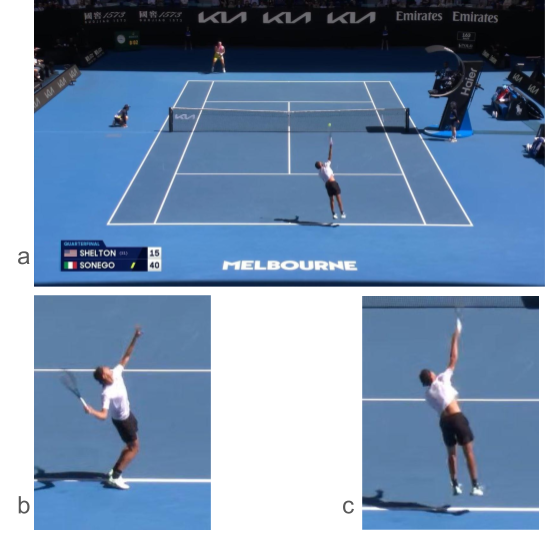
Individual images capturing the serves of eight tennis players in the quarter-finals and semi-finals of the 2025 Australian Open were obtained by capturing stills from the publicly available YouTube feed²⁸. All footage used was publicly accessible and analyzed under fair use for research purposes. At least 12 pairs of images were collected per player per match in both the quarter-finals and semi-finals, with service speed obtained from broadcast speed (km/h) based on radar (eg Figure 1).

Preprocessing

For the MediaPipe-based pose pipeline, frames were optionally preprocessed using contrast-limited adaptive histogram equalization (CLAHE) then lightly blurred with a Gaussian filter before pose inference. These steps were applied empirically to improve gross pose detection stability in broadcast footage characterized by variable lighting, compression artifacts, and motion blur. CLAHE served to enhance local contrast, while Gaussian blurring was used to suppress high-frequency noise that might otherwise destabilize keypoint regression.
Preprocessing was not applied to the YOLO-based pipeline, as preliminary inspection did not show a similar effect on pose outputs. No quantitative pose-accuracy validation was performed, and preprocessing is not claimed to improve joint-level accuracy. Instead, it was used as a practical robustness measure to reduce complete pose-estimation failures under challenging visual conditions.

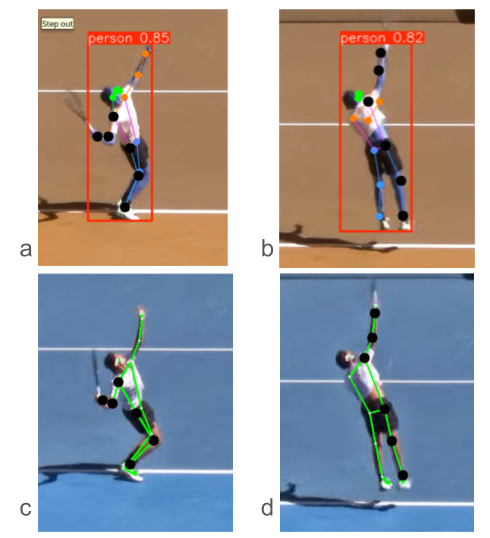
Because of noticeable motion blur, each pose model was visually checked to ensure that the joints matched the photograph correctly and that the dominant side and joints were properly identified. Manual inspection served only to remove major pose-estimation errors and was not applied as a quantitative measure of pose accuracy. A total of 213 out of 256 images were deemed acceptable for analysis in the YOLO method and 185 of 256 images by the MediaPipe method (Table 2A and 2B). Using joint position data, angles for the elbow, knee, hip and shoulder coil on the dominant side were calculated using 2D (YOLO) and 3D (MediaPipe) vector geometry. For the dominant wrist and shoulder, the Y-position was also used to measure elevation and arm extension. In the MediaPipe data, these values were normalized to torso length. Δ features were computed as the difference between the Extension and Loading phase angles.

Joint Angle Computation

Joint angles were computed from pose keypoints using standard geometric definitions. For each joint, the angle was calculated from three anatomically adjacent keypoints forming two vectors that meet at the joint of interest. Specifically, the elbow angle was defined by the shoulder–elbow–wrist triplet, the knee angle by the hip–knee–ankle triplet, and the hip angle by the shoulder–hip–knee triplet on the dominant side.

Given three points A, B, and C, where B represents the joint center, the joint angle θ was calculated as:

All angles were computed separately for each frame and used as input features for downstream classification tasks. Pose data were obtained using a YOLO-based keypoint detection model as well as Google’s MediaPipe pose analysis (see Table 1 for specific parameters of pose analysis). The shoulder coil angle was defined as a proxy for axial trunk rotation in the transverse plane. It was computed as the angle between the line connecting the left and right shoulder keypoints and the line connecting the left and right hip keypoints. Larger values indicated greater separation between shoulder and hip orientation, reflecting increased torso rotation during the loading phase of the serve.

Vertical limb position was defined as the normalized vertical coordinate (Y-position) of selected keypoints relative to the image frame. Specifically, the dominant wrist and dominant shoulder Y-coordinates were used to quantify limb elevation. For MediaPipe-derived features, vertical positions were normalized to torso length to account for differences in scale and camera perspective. Higher wrist Y-position values correspond to greater arm elevation during the serve motion.

Serve speeds were discretized within each athlete into three ordinal categories (Low/Medium/High) using tertile thresholds computed from that athlete’s observed serve speed values (33.3rd and 66.7th percentiles). Specifically, Low ≤ Q33, Medium between Q33 and Q67, and High ≥ Q67. Because broadcast radar speeds are discrete and ties may occur near cut points, exact bin counts can vary very slightly from equal thirds. Table 5 presents per-athlete speed distributions, cut points, and resulting class counts.

Classification Model Selection

Random Forest classifiers were used for all predictions. I had limited data given the time and nature of manual image extraction – Random Forest can perform well with limited data sets, in contrast to neural networks which could overfit a small data set. Random Forest accepts data with both heterogeneous features (eg joint angles, image heights) and does not require data to be normalized, and can output feature importance to the model, allowing me to understand which features were most important for prediction.

Model Configuration

All Random Forest models were implemented using the scikit-learn library. I used a standard approach for models: Random Forest models were trained with 500 decision trees, Gini impurity as the split criterion, and no explicit maximum tree depth. These settings were determined beforehand and were not adjusted using test data.

Feature Scaling and Class Imbalance

As Random Forest can accept data without feature normalization, no feature scaling or normalization was applied. For serve phase classification (loading/extension), there was minimal class imbalance so no reweighting was used. For ordinal serve speed classification (serve speed low/med/high), classes were defined using within-athlete tertile binning, which produced roughly balanced class distributions so no resampling or class-weighting methods were used.

Feature Importance Estimation

To estimate feature importance, I used the standard approach of using impurity-based (Gini) importance calculated during Random Forest training. These values were averaged across cross-validation folds to estimate the relative contribution of each feature to performance across the models. Other techniques to assess feature importance like permutation-based importance were not applied because of the limited nature of this dataset.

Validation Procedure

Model performance was evaluated using leave-one-athlete-out cross-validation. In each fold, the model was trained only on data from all but one athlete and tested on the held-out athlete, ensuring that no frames from the same athlete appeared in both training and test sets. Frames from the same serve sequence were kept together when identifiable. However, due to broadcast sampling, some correlation between visually similar frames or camera segments might still exist.

Parameter	YOLOv8-Pose (2D)	MediaPipe BlazePose (3D)
Dimensionality	2D (X,Y)	3D (X,Y,Z + visibility)
Model Source	Ultralytics YOLOv8 (PyTorch)	Google MediaPipe (BlazePose heavy)
Confidence Threshold	0.60	0.60
Keypoint Confidence	0.75	0.75
Input Mode	Static frame inference	Static image mode
Image Size	640 × 640 px	Original resolution (CLAHE preprocessing)
Pose Model Complexity	N/A	model_complexity = 2 (heavy model)
Angles Computed	Elbow, Hip, Knee, Shoulder Coil (2D)	Elbow, Hip, Knee, Shoulder Coil (3D)
Preprocessing	None (native YOLO resizing)	CLAHE + Gaussian Blur + Weighted Unmasking
Dominant Side Logic	Right (Left override for SHE)	Right (Left override for SHE)
Manual Review	Matplotlib interactive (1/2/3 keys)	Matplotlib interactive (1/2/3 keys)
Output Format	serve_pose_YOLO_FINAL_ANGLES_V2.csv	serve_pose_MediaPipe_3d_normalized_accepted.csv

Athlete	Loading	Extension	Total
Alex de Minaur	0	8	8
Alexander Zverev	9	22	31
Blake Shelton	3	22	25
Carlos Alcaraz	5	12	17
Jannik Sinner	9	19	28
Lorenzo Sonego	9	9	18
Novak Djokovic	20	21	41
Tommy Paul	10	7	17

Athlete	Loading	Extension	Total
Alex de Minaur	6	9	15
Alexander Zverev	10	21	31
Blake Shelton	17	21	38
Carlos Alcaraz	11	5	16
Jannik Sinner	17	18	35
Lorenzo Sonego	10	7	17
Novak Djokovic	21	22	43
Tommy Paul	10	7	17

Tables 2A and 2B summarize the number of images available per serve phase for each athlete in the MediaPipe 3D and YOLO 2D pipelines. Both systems captured a roughly balanced distribution of loading and extension frames per athlete.

The YOLO-based 2D extraction yielded slightly higher total frame counts (212 vs. 185), as MediaPipe often did not map the shoulder/elbow/wrist to the athlete, with greater intolerance for motion blur, leading the images to be manually rejected.

The balanced phase representation within each dataset supports the reliability of subsequent within-athlete classification and regression analyses.

Results

Cross-Athlete Phase Classification Results

We first evaluated whether pose-derived features extracted from broadcast footage could reliably distinguish between the Loading and Extension phases of the tennis serve and generalize across athletes. To assess cross-athlete generalization, a leave-one-athlete-out Random Forest model was trained on all athletes except one, then tested on the held-out individual. 

Both the YOLO (2D) and MediaPipe (3D) feature sets were used to predict whether a frame belonged to the Loading or Extension phase of the serve. Both the YOLO-based 2D feature set and the MediaPipe-based 3D feature set showed strong classification performance across athletes, with consistently strong F1 scores and ROC-AUC values for the binary phase classification task. 

These results indicated that pose-derived features extracted from broadcast images hold enough information to distinguish serve phases under standard viewing conditions.

System	Mean Accuracy	Mean F1	Mean ROC-AUC
MediaPipe 3D	0.989	0.993	1.000
YOLO 2D	0.985	0.987	0.999

Feature	MediaPipe 3D Importance (Mean ± SD)	YOLO 2D Importance (Mean ± SD)	Interpretation
Wrist Y-position	0.34 ± 0.03	0.47 ± 0.01	Vertical wrist position was the strongest discriminator of serve phase, reflecting racket elevation and arm extension changes.
Knee Angle	0.24 ± 0.03	0.13 ± 0.03	Captures lower-body drive and leg flexion-extension differences between phases.
Elbow Angle	0.23 ± 0.02	0.19 ± 0.02	Reflects arm flexion during loading versus near-full extension at impact.
Hip Angle	0.07 ± 0.02	0.13 ± 0.04	Represents trunk-pelvic alignment; modestly higher in YOLO due to projection effects.
Shoulder Coil Angle	0.11 ± 0.02	0.06 ± 0.02	Captures torso rotation; indicates moderate predictive role of upper-body torsion.
Shoulder Y-position	0.006 ± 0.003	0.018 ± 0.006	Minor role; shoulder elevation changes contribute little to phase discrimination.

Within-Athlete Ordinal Serve Speed Prediction

To see whether biomechanical features from single static images of serve (either loading or extension) are sufficient to predict serve speed, I used the extracted pose estimation data (both from MediaPipe 3D and YOLO 2D models). Each image had a corresponding serve speed (km/h) which was binned into low, medium, or high velocity categories based on athlete-specific quantile thresholds.

The data for the serve-speed distributions and the cut points are listed in Table 5. While this speed tertile binning generally produces balanced classes by design, there were deviations because of the rounded nature of radar speeds with some serves near or at boundary speeds. This condition can make some groups slightly uneven. Because the groups are slightly uneven, the majority class baseline ranged from 0.35-0.40 rather than the ideal value of 0.33 if the groups were perfectly balanced. Random forest classifiers were trained within each athlete using six pose-based predictors (elbow, knee, hip, shoulder-coil angles, and the vertical positions of the wrist and shoulder). In order to test the model’s prediction, for each athlete, I used five fold stratified cross-validation. The model was trained and tested five times using different train-test splits. The splits were stratified so each test would have a mixture of different speed categories. The average accuracy and F1 was reported.

Player	YOLO n	YOLO Q33	YOLO Q67	YOLO L/M/H	MP n	MP Q33	MP Q67	MP L/M/H
Alcaraz	16	148.0	188.0	7/4/5	17	146.0	194.67	6/5/6
De Minaur	15	162.0	192.0	5/ 5/ 5	8	165.67	192.67	3/2/3
Djokovic	43	158.0	186.0	14/15/14	41	146.67	186.0	14/13/14
Paul	17	147.0	160.67	6/5/6	17	147.0	165.0	6/ 5/6
Shelton	38	170.0	191.0	13/12/13	25	167.0	189.0	8/ 9/8
Sinner	35	157.0	182.0	12/11/12	28	157.0	166.0	9/10/9
Sonego	17	176.33	195.0	6 /5/ 6	18	172.67	195.0	6/ 6/6
Zverev	31	197.0	206.0	10/13/8	31	178.0	206.0	10/11/10

Model	Athletes	Accuracy	Baseline	Δ Accuracy	Macro-F1
YOLO Static	8	0.336	0.380	−0.044	0.293
MediaPipe Static	7	0.318	0.331	−0.013	0.274
YOLO Δ	4	0.456	0.385	+0.072	0.389
MediaPipe Δ	2	0.435	0.393	+0.042	0.405

Overview of Model Performance

To evaluate model performance, I compared each model to a simple baseline that always predicted the most common serve-speed category for that athlete. This provided a more meaningful benchmark than comparing the results to the theoretical chance level of 0.33, because the speed categories were not perfectly balanced (table 5). Performance was measured using accuracy and macro-F1, and summarized at the athlete level.

A summary comparison of static (pose-based) and temporal (Δ-feature) models across athletes is shown in Table 6.

Across all athletes, static pose-based models did not outperform the baseline. Mean accuracy for YOLO-based static features was 0.336 compared to a baseline of 0.380, and MediaPipe-based static features also fell below baseline (0.318 vs 0.331). These values are close to the theoretical chance level for a three-class problem (0.33), suggesting that a single still image does not contain enough information to predict serve speed.

In contrast, models incorporating paired images of loading/extension with changes between images (Δ features) demonstrated modest but consistent improvements over baseline. YOLO-derived Δ features achieved a mean improvement of +0.072 accuracy above baseline, while MediaPipe-derived Δ features showed a smaller but positive improvement (+0.042). The F1 score assesses how the model performed across each class rather than only the number of correct predictions. The models incorporating temporal differences also had higher F1 scores, suggesting better performance across all classes rather than simply predicting the most common serve speed category.

Paired within-athlete comparisons

To make a fair comparison between the Δ features and static model, I only included athletes who had enough data for both models. Across these athletes with adequate data (n = 4), YOLO Δ models outperformed YOLO static models by an average of +0.084 accuracy relative to baseline. This suggests that changes between the loading and extension phases contain more information about serve speed than a single still image. Comparisons between MediaPipe static and Δ models were inconclusive, only two athletes had adequate data, and there was no consistent improvement observed (-0.013). The results suggest that using the Δ features may improve prediction compared with a single still image. However, this advantage was modest and depended on how many athletes had enough data for analysis.

Sensitivity to minimum sample size

To assess robustness, analyses were repeated across increasing minimum sample thresholds per athlete (MIN_N = 12, 15, 20). Increasing the threshold reduced the number of included athletes but did not reverse the observed pattern.

At higher thresholds (MIN_N = 20), the number of evaluable athletes decreased substantially, particularly for Δ-feature models, resulting in limited overlap across models (n = 1). However, in the remaining high-sample athlete, Δ-feature models continued to outperform static models (e.g., YOLO Δ accuracy 0.476 vs YOLO static 0.402).

These results imply that the observed advantage of Δ features is not solely driven by low-sample athletes, although statistical power is reduced at higher thresholds.

Inter-athlete variability

Substantial variability in performance was observed across athletes for all models. For example, static YOLO accuracy ranged from approximately 0.20 to 0.45 across athletes, reflecting heterogeneous predictive difficulty.

To measure this variability, model performance was evaluated at the athlete level and compared using paired differences relative to baseline. The standard deviation of accuracy across athletes ranged from 0.055 to 0.102 for static models and 0.058 to 0.130 for Δ models, showing considerable inter-athlete heterogeneity.

Given the limited number of athletes, formal statistical inference is constrained; however, paired comparisons consistently showed positive directional effects for Δ features relative to static features, supporting the presence of a modest but systematic signal.

Interpretation of model performance

Overall, none of the serve speed prediction models achieved high accuracy – most classified fewer than half the serves correctly. Predicting whether a serve is slow, medium or fast for the same player is a difficult task using only the pose measurements from broadcast images.

Importantly, pose measurements from static images alone did not provide predictive results better than guessing the most common class (strict baseline). In contrast, changes in pose from loading to extension (Δ features) showed modest but consistent improvements beyond chance. These findings suggest that the way a player moves from loading to extension contains more relevant information than static posture for serve speed.

Discussion

This study used biomechanical features extracted from still images of a broadcast tennis match for two different tasks. The first task was whether this data could be used for phase classification across athletes and the second task was whether this data could be used for within athlete ordinal serve speed prediction. These tasks had very different results, with phase classification being much more successful than serve speed prediction.

Phase Classification Discussion

Both the Mediapipe 3D and YOLO 2D models successfully classified static images as Loading versus Extension across athletes. Near perfect performance was obtained even when the models were tested on athletes excluded from training, suggesting that the pose-derived patterns distinguishing these phases are similar across athletes.

The near perfect performance of this classification task (ROC-AUC near 1) is likely related to the simplicity of differentiating these two phases rather than confirmation that precise joint centers or angles can be extracted from broadcast still images. This near perfect result in classification across athletes suggests that the extracted features, including limb elevation and joint configuration, are sufficient to reliably differentiate phases even with varying camera parameters and motion blur.

These results imply that serve phase classification from broadcast video is a relatively coarse and visually distinct task that remains robust against pose estimation noise.

Within-Athlete Ordinal Serve Speed Prediction

In contrast to phase classification, serve speed prediction proved considerably more challenging. Static pose-based models reached mean accuracies close to baseline levels, showing limited separation from majority-class baselines across athletes. This suggests that single frame biomechanical features contain little predictive information for ordinal serve speed classification in this context. These findings align with the expectation that serve speed depends on coordination, sequencing and temporal energy transfer rather than any single static posture that can be captured in isolated frames^3,4.Additional three dimensional analyses have measured the contributions of individual joint rotation to racquet speed during the serve, further supporting the view that serve velocity reflects coordinated multi-joint movement rather than a single static position⁵.

Incorporating temporal features, defined as differences between Loading and Extension frames (Δ features), led to modest yet consistent improvements compared with strict baselines. Paired within-athlete comparisons demonstrated that YOLO Δ outperformed corresponding static models by approximately +0.084 accuracy relative to baseline across shared athletes. Although absolute performance remained low (generally <0.50 accuracy), these directional improvements were consistent across analyses and persisted across minimum sample size thresholds (12,15,20 serves). This supports the presence of a weak but systematic signal linked to temporal biomechanical change, consistent with prior work suggesting that dynamic representations are better suited than static postures for multi-joint movement analysis²⁶ and that temporal pose representations can improve movement modeling compared with isolated frames²⁷.

Differences in performance between YOLO and MediaPipe models should be viewed in light of data availability and representation. The MediaPipe model produced fewer usable frames for several athletes and exhibited greater class imbalance (for example, limited or absent Loading-phase frames in some cases), which likely reduced model stability in within-athlete analyses. Given the small sample sizes and three-class classification setting, these differences in data quantity and balance are expected to have a substantial impact on performance.

In addition, MediaPipe’s 3D reconstruction depends on depth inference from single camera broadcast footage, which may introduce extra noise under conditions of motion blur, occlusion, and variable camera geometry²⁹. While this provides a plausible reason for reduced performance relative to 2D keypoint representations, the current study does not separate representation effects from differences in sample size. Therefore, the relative influence of data quantity versus 3D reconstruction noise cannot be determined with certainty.

Substantial inter-athlete variability was observed across all models, with accuracy ranging widely within each feature set. This heterogeneity likely reflects differences in serve mechanics, consistency of motion patterns, and sample size. While formal statistical testing is limited by the small number of athletes, the observed variability underscores the challenge of generalizing biomechanical prediction models even within controlled, intra-athlete settings.

Several factors likely contributed to the overall low predictive performance. Because all source footage was derived from publicly available YouTube broadcasts, each athlete occupied only a 640 × 640 pixel region of the cropped image, limiting the spatial resolution of pose detection. Moreover, many frames exhibited motion blur of the dominant arm given the speed of motion during the serve, resulting in loss of joint fidelity and rejection of a substantial proportion of images during quality control. These factors likely constrained both angular accuracy and the stability of derived 3D coordinates. Furthermore, the feature set was limited to a small number of joint angles and vertical position measures, which may not fully capture the biomechanical determinants of serve velocity including joint rotation contributions, upper limb segment rotations, lower limb force production, service side variations and kinetic chain interactions^5,30,7,10. Lastly, the use of frame pairs rather than continuous motion sequences restricts the ability to model temporal dynamics in a more complete way.

These findings position the current work as an exploratory analysis of the feasibility of using broadcast-derived pose features for serve speed prediction. While static features were insufficient for meaningful prediction, temporal differences between key serve phases provided modest gains, suggesting that dynamic biomechanical information is necessary but not sufficient in this formulation. These results should be interpreted as exploratory and not intended to show generalizable predictive modeling.

Future work should focus on improving both data quality and feature representation. Higher-resolution, high-frame-rate video could reduce motion artifacts and improve pose estimation fidelity. Incorporating full temporal sequences rather than discrete frame pairs may allow modeling of coordination patterns and energy transfer.

References

1. Martin C. Biomechanics of the tennis serve. Tennis medicine: a complete guide to evaluation, treatment, and rehabilitation. 2019. [↩] [↩]
2. Elliott, B. “Biomechanics and Tennis.” British Journal of Sports Medicine 40 (2006): 392–396. [↩]
3. Fleisig, Glenn, Rochelle Nicholls, Bruce Elliott, and Rafael Escamilla. “Kinematics Used by World Class Tennis Players to Produce High-Velocity Serves.” Sports Biomechanics 2, no. 1 (2003): 51–64. https://doi.org/10.1080/14763140308522807. [↩] [↩]
4. Bahamonde, R. E. “Changes in Angular Momentum during the Tennis Serve.” Journal of Sports Sciences 18, no. 8 (2000): 579–592. [↩] [↩]
5. Gordon, B. J., and J. Dapena. “Contributions of Joint Rotations to Racquet Speed in the Tennis Serve.” Journal of Sports Sciences 24, no. 1 (2006): 31–49. [↩] [↩] [↩]
6. Fenter, B., T. S. Marzilli, Y. T. Wang, X. Dong. “Effects of a Three-Set Tennis Match on Knee Kinematics and Leg Muscle Activation during the Tennis Serve.” Perceptual and Motor Skills 124 (2017): 214–232. https://doi.org/10.1177/0031512516672773. [↩]
7. Girard, O., J. P. Micallef, and G. P. Millet. “Lower-Limb Activity during the Power Serve in Tennis: Effects of Performance Level.” Medicine & Science in Sports & Exercise 37, no. 6 (2005): 1021–1029. https://doi.org/10.1249/01.mss.0000171619.99391.bb. [↩] [↩]
8. Kwon, J. W. “A Conceptual Field-Based Framework for Lower-Upper Body Kinetic Chain Assessment in the Tennis Serve Using IMUs and Portable Force Plates: Measurement Coverage, New Performance Indices, and Applied Implications.” Frontiers in Sports and Active Living 8 (2026): 1784684. [↩]
9. Whiteside, D., B. Elliott, B. Lay, and M. Reid. “A Kinematic Comparison of Successful and Unsuccessful Tennis Serves across the Elite Development Pathway.” Human Movement Science 32, no. 5 (2013): 822–835. https://doi.org/10.1016/j.humov.2013.06.003. [↩]
10. Fett, J., N. Oberschelp, J. L. Vuong, J. Wiewelhove, and A. Ferrauti. “Kinematic Characteristics of the Tennis Serve from the Ad and Deuce Court Service Positions in Elite Junior Players.” PLOS ONE 16, no. 7 (2021): e0252650. https://doi.org/10.1371/journal.pone.0252650. [↩] [↩]
11. Huesca-Flores S et al. Skeleton-based baseball pitch classification on broadcast videos. SPIE. 2025. [↩]
12. 12. P. Jafarzadeh, L. Zelioli, P. Virjonen, F. Farahnakian, P. Nevalainen, J. Heikkonen. Enhancing hurdles athletes’ performance analysis: a comparative study of CNN-based pose estimation frameworks. Multimedia Tools and Applications. Vol. 84, pg. 34573-34591, 2025, DOI: 10.1007/s11042-024-20587-z. [↩]
13. L. Liu, Y. Dai, Z. Liu. Real-time pose estimation and motion tracking for motion performance using deep learning models. Journal of Intelligent Systems. Vol. 33, pg. 20230288, 2024, DOI: 10.1515/jisys-2023-0288. [↩]
14. M. Habibi, M. Nourani, M. Nourani. AI-based kinematic analysis for track athletes. 2024 IEEE International Conference on Smart Computing. pg. 338-343, 2024, DOI: 10.1109/SMARTCOMP61445.2024.00078. [↩]
15. T. Surasak, P. Temjai, P. Wilaikaew, K. Kitchat, S. Thongrattana. Advanced golf swing analysis using MediaPipe and machine learning. In Ubi-Media Computing, Pervasive Systems, Algorithms and Networks. pg. 299-314, 2025, DOI: 10.1007/978-981-96-6291-3_24. [↩]
16. L. Huang, J. Chen. Basketball dribbling action recognition and performance evaluation based on YOLO-Pose and LSTM. Proceedings of SPIE. Vol. 14115, pg. 141151B, 2026, DOI: 10.1117/12.3102702. [↩]
17. Lyu, Y., X. Duan, C. Yang, and Q. Ye. “Development of a MediaPipe-Based Framework for Biomechanical Quantification of Table Tennis Forehand Strokes.” Frontiers in Sports and Active Living. 2025. [↩]
18. Edriss, S., C. Romagnoli, M. Maurizi, et al. “Pose Estimation for Pickleball Players’ Kinematic Analysis through MediaPipe-Based Deep Learning: A Pilot Study.” Journal of Sports Sciences. 2025. [↩]
19. Wei, X., P. Lucey, S. Morgan, P. Carr, M. Reid, and S. Sridharan. “Predicting Serves in Tennis Using Style Priors.” In Proceedings of the 21st ACM SIGKDD International Conference on Knowledge Discovery and Data Mining, 2015. [↩]
20. Whiteside, D., and M. Reid. “Spatial Characteristics of Professional Tennis Serves with Implications for Serving Aces: A Machine Learning Approach.” Journal of Sports Sciences 35 (2017). [↩]
21. Vives, F., J. Lázaro, J. F. Guzmán, and R. Martínez-Gallego et al. “Optimizing Sporting Actions Effectiveness: A Machine Learning Approach to Uncover Key Variables in the Men’s Professional Doubles Tennis Serve.” Applied Sciences 13 (2023). [↩]
22. Zhu, Y., and R. Naikar. “Predicting Tennis Serve Directions with Machine Learning.” 2022. [↩]
23. Tea, P., and T. B. Swartz. “The Analysis of Serve Decisions in Tennis Using Bayesian Hierarchical Models.” Annals of Operations Research (2023). [↩]
24. Kovalchik, S., and M. Reid. “A Calibration Method with Dynamic Updates for Within-Match Forecasting of Wins in Tennis.” International Journal of Forecasting 35 (2019). [↩]
25. Gao, Z., and A. Kowalczyk. “Random Forest Model Identifies Serve Strength as a Key Predictor of Tennis Match Outcome.” Journal of Sports Analytics 7 (2021). [↩]
26. Mateus R et al. Static vs dynamic optimization in biomechanics. Springer. 2020. [↩] [↩]
27. Li Z, Li Z. Deep learning-based pose estimation. Sci Rep. 2025. [↩] [↩]
28. Australian Open TV YouTube channel. [↩]
29. Ferraris, C., G. Amprimo, S. Cerfoglio, L. Vismara, and V. Cimolin. “A Deep Dive Into MediaPipe Pose for Postural Assessment: A Comparative Investigation.” IEEE Access 13 (2025): 211055–211074. https://doi.org/10.1109/ACCESS.2025.3643126. [↩]
30. Elliott, B. C., R. N. Marshall, and G. J. Noffal. “Contributions of Upper Limb Segment Rotations during the Power Serve in Tennis.” Journal of Applied Biomechanics 11, no. 4 (1995): 433–442. https://doi.org/10.1123/jab.11.4.433. [↩]