
Abstract
Street lighting is amongst the most energy-intensive municipal services, since most installations run at a fixed static output throughout the night regardless of conditions. This study asks whether streetlight-power demand can be predicted from weather, traffic, and temporal context, and whether such a model can drive an adaptive-dimming controller that can reduce consumption by a significant figure. Feeder-level data from twelve smart-lighting controllers in Delhi (30 Nov 2024 to 31 Mar 2025; approximately 143,800 fifteen-minute records). A leakage audit shows that the electrical channels reconstruct active power through the identity that active power equals voltage times current times power factor, at an R-squared value of 0.9998. All thirty-eight such features were removed and a Random Forest model was retrained on only contextual features under a strict chronological eighty-twenty train-test split. It can predict active power with a mean absolute error of 1.01 kilowatts, and R-squared value of 0.895. This is the best RMSE and R-squared value amongst all the tested models, with gradient boosted trees having a slightly lower MAE of 0.98 kilowatts. Weather and traffic only improve the prediction accuracy modestly. Coupled to a luminance-anchored dimming controller whose floor value equals the ratio of the two road-lighting classes’ luminances, it is then verified that road luminance never falls below the class minimum. On the held-out month, it reduces operating-hour power by about twenty-nine percent, reproduced on actual metered power, while remaining fully luminance-compliant. It is concluded that the value of the added data lies in enabling demand-aware control.
Keywords: adaptive street lighting, power-demand prediction, Random Forest regression, data leakage, chronological validation, demand-responsive dimming, road-lighting luminance class, energy efficiency.
Introduction
In recent years urban electricity demand has risen sharply with economic and population growth, placing public lighting as one of the largest controllable loads that a municipality manages1. Conventionally, these installations are static: the lamps switch on at dusk, holding a fixed output till dawn, irrespective of any factor such as traffic, weather, or pedestrians, which wastes energy during the various low-activity hours at night. The reported figures for the share of municipal electricity bills which is attributable to public lighting varies greatly with city size and its electrification, and the often-quoted forty-to-sixty percent range1 should be taken as an upper-bound estimate for those municipalities which are lighting heavy rather than as a universal constant; we therefore treat it in an indicative context.
A recurring ambiguity in this literature is the conflation of the two distinct problems. The first is prediction: the estimation, from observable conditions, of how much power a lamp will draw. The second is control: deciding how bright a lamp should be set depending on the time of day. A model that predicts demand under the current control regime does not, by itself, prescribe the dimming actions, and much of the prior work blurs this important distinction.
Therefore, the research question is twofold: (i) to what extent can feeder-level streetlight power be predicted from the contextual features alone, once all the features that trivially determine the target are removed; and (ii) can the resulting model be used, within a safety floor constraint expressed in photometric terms, to create a dimming policy that is capable of demonstrating energy use reduction. Our working thesis is that the contextual prediction is accurate enough that it can support scheduling and control, but that the contextual features add little to point accuracy beyond the day-night signal, so their value is instead realised in control rather than in regression.
Contributions. This paper makes the following contributions:
- It diagnoses and removes a data-leakage pathway that had a near-perfect accuracy (R-squared 0.9998) and establishes an honest performance baseline under a strict chronological train-test split.
- It quantifies, by ablation, the genuine marginal value of weather and traffic features for the purpose of power prediction, rather than asserting an improvement.
- It couples the demand model to a luminance-anchored dimming controller in which the model gates operation and supplies the demand baseline, closing the prediction-to-control gap.
- It anchors the dimming floor value for a road-lighting class and verifies, by a luminance check, that the dimmed floor value never falls below the class safety minimum.
- It reports an energy saving that is validated out-of-sample against actual metered power and frames it honestly as a simulation which awaits field-deployment.
The scope is deliberately limited to a single four-month, cool-season dataset of two different Delhi localities, and to a simulated controller rather than to a hardware deployment; these limitations are stated explicitly in the text and are further revisited in the discussion.
Related Work
The work relevant to this study spans six strands: class-based dimming evaluated in the field; sensor-driven and networked control architectures; learning-based control; machine-learning forecasting of electrical demand; weather and traffic as predictors; and the photometric basis for dimming safely. These strands report their results on terms that are not directly comparable: the baselines, the observation windows, and the measurement rigour all differ, the last of these ranging from full metering through to pure simulation. Therefore, the review below groups the prior work by what it actually demonstrates rather than by how much saving it claims, and Table 1 records, for each representative study, the limitation that matters most here.
Class-Based and Field-Measured Adaptive Lighting
Large-scale municipal implementations following the EN 13201 and the UNI 11248 report energy savings of about 48%, reaching a max ceiling of nearly 70% upon reducing lighting classes during low traffic periods1,2,3. Similar class-based studies show that the savings are largely a product of how far lighting can be reduced, with real-world pilots reporting reductions up to 80%2,4,3,5. Long-term monitoring shows that simulated assumptions differ from the actual maintenance conditions and photometric performances6,1,3. The study that is closest to the present work uses forecasted traffic data to drive dimming and reduce electricity consumption. It predicts traffic rather than electrical demand and does not report any forecast accuracy7.
Sensor-Driven and Networked Control Architectures
Real-time hybrid models that use traffic, weather, and low-power communication report energy savings of about 55%, but they are mainly evaluated through hardware deployment and have limited statistical analysis8,9,10. Larger municipal systems integrate both smart metering and illumination control, though most of the savings are a product of regulation and scheduling rather than of demand-responsive dimming11,10,4,5.
Learning-Based Control
Reinforcement learning is commonly used to reduce lighting energy while still maintaining illuminance, though the work takes place indoors12. Outdoor predictive control does exist, but it heavily relies on explicit models and sensing13,7. Feeder-scale control using policies that are driven directly by demand forecast remain largely unexplored here12,13,7,14.
Machine-Learning Demand Forecasting
Random Forest performs competitively in short-term load forecasting, with traffic data offering smaller gains as compared to temporal features15,16,17. The adaptive-lighting strand tends to build controllers with no demand model behind them, while the forecasting strand tends to build demand models that are never carried through to a controller10,11,15,16. This study connects the two.
Weather and Traffic as Predictors
Prior studies show that the electricity demand is affected by temperature, humidity, and solar radiation, though the solar radiation is largely confounded with time of day18,19,20,21,22. Short-term forecast accuracy in warm climates is also influenced by temperature, while deep-learning models are able to provide high-resolution flow estimation for urban networks19,23,17,18.
Photometric Anchoring and the Safety of Dimming
A dimming policy is only defensible if the reduction is bounded by a photometric criterion and not by some arbitrary power figure24,25,1,2. Work on mesopic vision shows that road-lighting energy can be optimised against luminance-based criteria while the visibility is preserved25,24,2. Experimental work on luminance reduction under mesopic photometry finds the high-acuity task performance to be preserved as long as it remains before a certain threshold, hence the floor has to be expressed in candela per square metre24,25. On a policy scale, a large controlled interrupted time-series evaluation across England and Wales found there to be no clear evidence that reduced street lighting, including both dimming and part-night regimes, increased crime or casualties26. In total, these justify usage of a conservative, class-anchored floor rather than an unconstrained optimisation24,25,26,1,2.
| Study (representative) | Method | Setting / data | Reported saving | Limitation relevant here |
| Pasolini et al. (2024)1 | Class-reduction dimming under EN 13201 / UNI 11248 | Measured municipal pilots (e.g., 878 lamps) | ~48% measured; up to 70% by class reduction | Requires real-time sensing; standard-specific |
| Takruri et al. (2023)8 | Traffic + weather dimming over NB-IoT | Experimental deployment | Up to ~55% | Hardware-specific; limited statistical evaluation |
| Gagliardi et al. (2020)4 | IoT adaptive control architecture | Two real pilot sites | Up to 80% vs traditional lighting | Architecture and baseline are pilot-specific |
| Wojnicki et al. (2019)2 | Lighting-class-based dynamic control | Computational road models | Class-dependent | Simulation only |
| Valetti et al. (2023)6 | Long-term photometric and energy monitoring | Multi-year LED field campaign | Degradation and maintenance quantified | Control effects and retrofit are intertwined |
| Krizanovic et al. (2026)3 | ML-based savings-assessment framework | Adaptive lighting scenarios | Framework for evaluating achieved savings | Not a demand model, only assessment method |
| Belloni et al. (2024)7 | Dimming driven by forecasted traffic | Road case study | Reduction vs fixed schedule | No accuracy metrics, forecasts traffic instead of demand |
| Mohandas et al. (2019)5 | Neural-network control | Residential area, Hosur, India | Case-study saving | Only tested on small area, no temporal validation |
| Sanchez-Sutil and Cano-Ortega (2021)11 | Smart regulation over LoRa LPWAN | Designed and experimentally evaluated system | Improved regulation and efficiency | No demand forecasting; direct control |
| Shaheen et al. (2026)13 | Model predictive control | Adaptive street-lighting case study | Energy-efficient control under changing conditions | Requires explicit model and sensing |
| Chaianong et al. (2022)17 | Random Forest load forecasting | Two Swiss distribution-grid areas | Traffic helps, but far less than time variables | Load is residential, not street lighting |
| Dudek (2022)15 | Random Forest short-term load forecasting | Public load series | Competitive accuracy reported | No control loop; only forecasting |
| This study | Leakage-controlled RF demand model + luminance-anchored dimming | 12 feeders, Delhi, 4 months, metered | ~29% operating-hour (validated out-of-sample, simulated control) | Single season; typical traffic; not yet field-metered |
Methods
Data
The dataset used for this study comprises reading from twelve feeder-level smart-lighting controllers in Delhi, India, which are logged at approximately fifteen-minute intervals from 30th November 2024 to 31st March 202527. Seven of these controllers serve in a residential locality (Laxmi Nagar), and five in a commercial locality (Mayur Vihar). After removing all the records with missing timestamps or targets, approximately 143,800 readings remain amongst these controllers. Each of these records reports: the target, total active power in kilowatts, electrical channels (per-phase and aggregate voltage, current, active, reactive, and apparent power, power factor, frequency, energy, and run-hour), and contextual channels. The magnitude of the per-controller load (medians of twelve to eighteen kilowatts) indicated that each unit meters a street segment consisting of multiple luminaires rather than just a single lamp.
The feeder power and electrical readings serve as the primary sensor data; the on-board temperature and humidity channels were disregarded as they were inoperative (constant zero value). Instead, the environmental context was obtained from a public weather server (Open-Meteo hourly analysis for the site coordinates: temperature, relative humidity, rain, cloud cover, visibility, sunshine duration, and shortwave solar radiation)28, and traffic context from a Delhi congestion profile (a typical weekday-by-hour congestion index and a monthly level)29.
Feature Set and Leakage Control
Running a sanity check confirmed that the target was being reconstructed algebraically by the electrical channels. The sum of the three per-phase active powers reproduces total active power at an R-squared of 0.9998, and the apparent power is multiplied by the magnitude of the power factor, which reproduces it at 0.9985; both follow from the identity: active power equals voltage times current times power factor. A model which is given these electrical channels learns arithmetic, not context, and an R-squared near unity is therefore trivial. All thirty-eight such electrical features were removed. The retained predictors are the external weather variables, two traffic variables, cyclic encodings of hour-of-day and day-of-year (sine and cosine), a binary precipitation flag derived from rain, one-hot encodings of the controller identity and locality, and a day-of-week index and weekend flag. A complete feature list containing the rationale for each engineering decision is provided later in the Appendix.
Chronological Split and Demand Model
Since the data forms a time series, a strict chronological split was used: the earliest eighty percent of readings (30th November 2024 to 7th March 2025) for the training, and the remaining final twenty percent (7th March to 31st March) for the testing, with no shuffling, to ensure that every test timestamp follows every training timestamp. This in turn avoids the leakage that a random eighty/twenty split introduces when adjacent readings from the same night are divided amongst the train and test. The hyperparameters were tuned by grid search under a time-series cross validation, to preserve ordering within each fold. The predictor is a Random Forest of three hundred trees that are regularised to a maximum depth of sixteen with a minimum of five samples per leaf; regularisation was added specifically to reduce the gap between train and test.
Baselines
The model is compared against four baselines on the same held-out month: an hour-of-day mean, a gradient-boosted-tree regressor, a static rated-power schedule, and an ordinary linear regression on the same features.
Operating-Schedule Characterisation
To characterise the system under control, the daily turn-on and turn-off times were estimated. From December to March, the evening turn-on drifts about seventy minutes later, closely tracking the seasonal sunset shift, and the morning turn-off drifts earlier with sunrise. This pattern shows no response to same-day cloud cover, which indicates that a pre-programmed astronomical schedule is being followed rather than live light sensing. Once on, these lamps draw an almost constant power, confirming that the present installation undergoes no intensity dimming; this is the headroom that the controller targets.
Closed-Loop Control Architecture
The predictor and the controller are linked together as follows. The operating window is decided by the model’s forecast of demand: a lamp is treated as operating when the predicted power exceeds a certain threshold, so the predictor inherits the dawn-to-dusk logic from the radiation, identity, and time features it uses. During operation, the dimming policy sets the intensity between a floor and full output as a function of demand and safety conditions: with rise in traffic congestion, intensity rises from the floor to full output, it is boosted to full output when the atmospheric visibility falls down into the haze range, and is reduced to the floor in dense fog based on the principle that strong light backscatters and does not aid in visibility. The controlled power is the predicted baseline scaled by an intensity-to-power map that includes a fixed driver overhead of ten percent so that savings are conservative. The saved energy is the difference between the predicted baseline and the controlled power. Therefore, the predictor contributes the operating-window forecast and the demand baseline that make the schedule deployable from a forecast; the magnitude of the savings is determined by the safety-bounded control policy.
Luminance-Class Anchoring and Safety Check.
Illumination standards specify a minimum maintained luminance, in candela per square metre, for each road-lighting class, not as an absolute power expressed in kilowatts; this conversion depends on fixture, mounting height, and on road geometry. Accordingly, the dimming floor value is expressed as a luminance ratio, rather than as a fixed power. Taking a design class of M3 (1.00 candela per square metre at full output) and a permitted night-minimum class of M5 (0.50 candela per square metre) from the EN 13201 / CIE 115 ladder and noting the fact that road-surface luminance scales with luminous flux, the floor being their ratio, fifty percent30. A luminance check then computes the realised luminance at every operation hour as intensity times design-class luminance and verifies that the luminance never falls below the class minimum; since intensity is bounded at the lower end by the floor, compliance is guaranteed for construction and is reported explicitly. For simplicity, for both the localities, a single common class is assumed; in practice, the class, and hence the floor, should differ by road type. The Indian standard IS 1944 provides the national analogue, expressed in lux by road group, and the same ratio method applies to those values31.
Energy-Savings Estimation and Ethics
On the held-out month, two saving figures are reported: a planned saving is computed from the model’s forecast baseline, and a realised saving is computed by applying the identical policy to the actual metered power. Agreement between these validated that the forecast-driven plan is achievable on unseen data. This study uses secondary feeder level data and public environmental and traffic data; it involves no human participation, and no personally identifiable information is used.
Results
Leakage Confirmation
The algebraic identities reproduce the target almost perfectly (R-squared of 0.9998 for the sum of the phase powers), confirming that a near perfect accuracy like such results from data leakage and reflects use of arithmetic modelling instead of a context-aware one. All such features have been excluded from the model reported below.
Prediction Performance and Overfitting
On the held-out month, the Random Forest is able to achieve a mean absolute error of 1.01 kilowatts, a root-mean-square error of about 2.5 kilowatts, and an R-squared value of about 0.895. This is the best RMSE and R-squared value amongst all the tested models, with gradient boosted trees having a slightly lower MAE (0.98, as opposed to 1.01) as is showcased and summarised in Table 2.
| Model | MAE (kW) | RMSE (kW) | R² |
| Static rated power | 19.41 | 20.84 | — |
| Hour-of-day mean | 3.79 | 5.54 | 0.466 |
| Linear regression | 3.77 | 4.53 | 0.644 |
| Gradient-boosted trees | 0.98 | 2.72 | 0.872 |
| Random Forest (this study) | 1.01 | 2.46 | 0.895 |
Regularisation was able to reduce the train-to-test mean-absolute-error ratio to about 1.4 (training error near 0.7 kilowatt against test error near 1.0 kilowatt), down from roughly 1.9 in an unregularized model, indicating mild residual overfitting with acceptable generalisation, since the test error matched the cross-validated error. A note on the metrics: the mean absolute percentage error is inappropriate here because half of all the records are daytime values near zero, which makes the percentage error diverge; restricted to operating hours, it is 11%. Therefore, the primary metrics reported are mean absolute and root-mean-square errors (in kilowatts).
Marginal Value of Weather and Traffic
Re-fitting with and without the external features, holding the model fixed, improves mean absolute error by about two percent, root-mean-square error by about four percent, and R-squared by about 0.009. Therefore, the added features deliver only a modest gain, concentrated in the harder high-power cases rather than the median, and are hence best described as confirming the demand signal rather than transforming the prediction accuracy.
Feature Importance
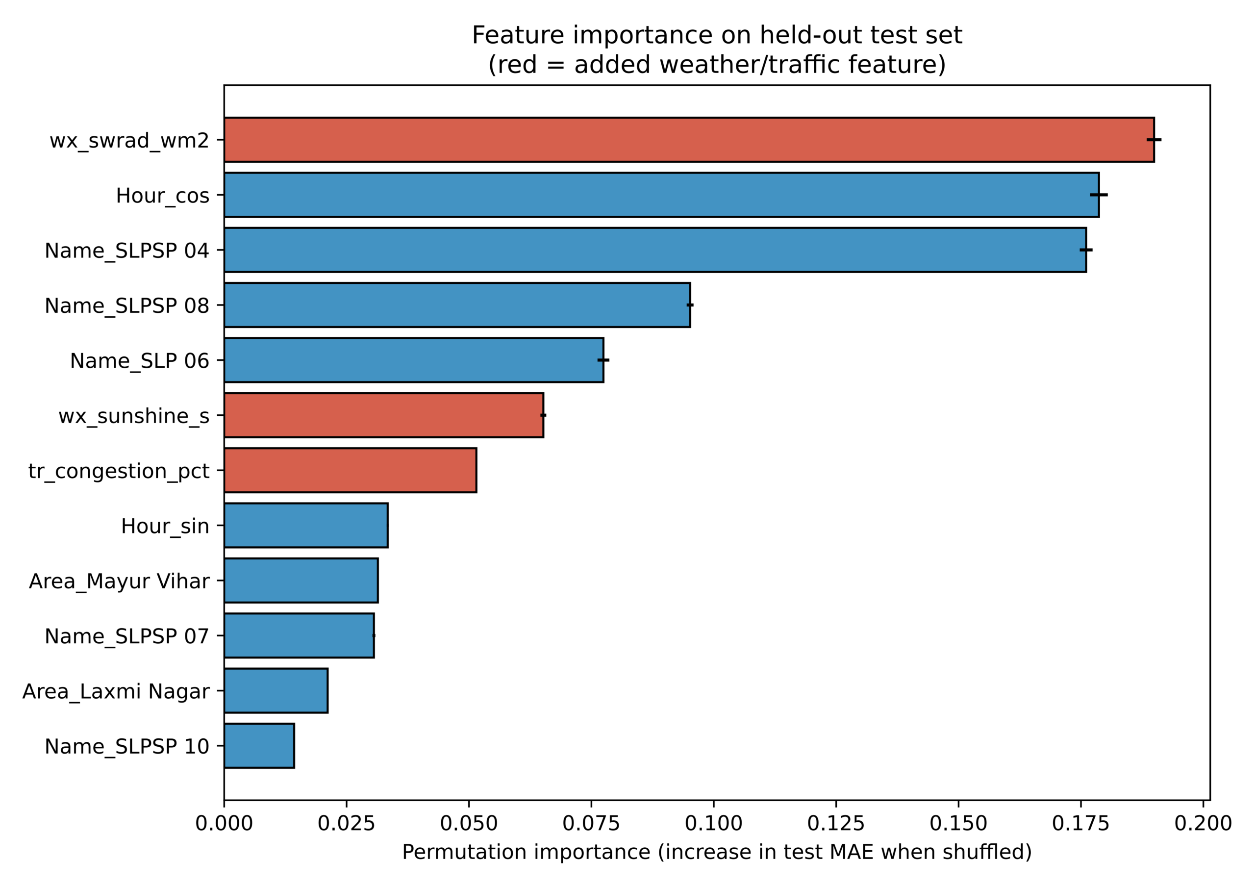
Using a permutation importance on the test set ranks solar radiation as first, followed by hour-of-day, several controller identifiers, sunshine duration, and traffic congestion. Visibility, cloud, temperature, rain, humidity, grid frequency, and precipitation flag carry essentially no importance (Figure 1). The leading rank of solar radiation is a collinearity artefact: in a model without weather, the hour-of-day cosine alone carries the day-night signal, and adding radiation, which also encloses whether it is dark, just merely redistributes that importance. Traffic congestion correlates equally with power and with hour-of-day, so its apparent value is largely determining the time-of-day. None of the contextual features are leaky, as all are exogenous to the meter.
Stratified Held Out Evaluation
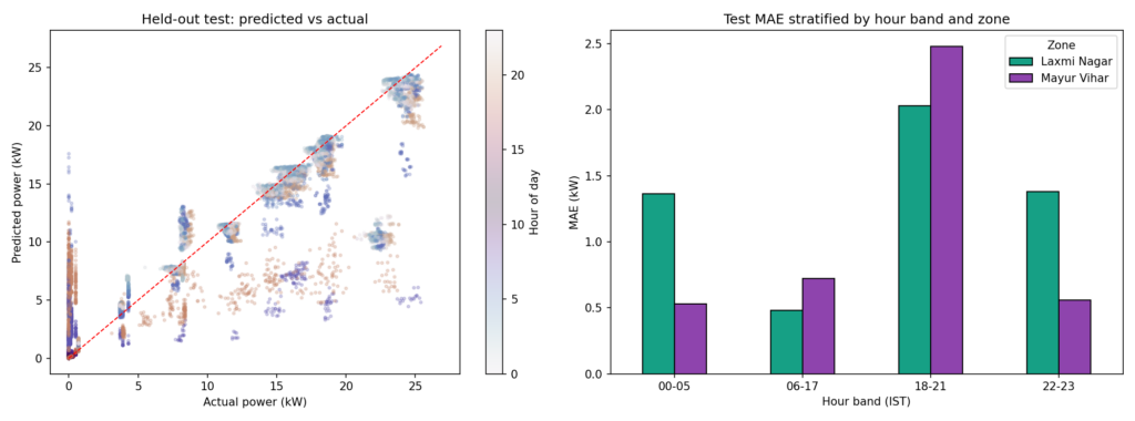
Figure 2 presents the held-out distribution of predicted vs actual power and the mean absolute error stratified by hour band and locality. The error is mostly concentrated in the evening peak (eighteen to twenty-one hours), where power is highest and most variable, and is far smaller during the daytime-off and deep-night periods; the commercial locality shows slightly higher peak-hour error than the residential one does.
Closed-Loop Savings and Luminance Compliance.
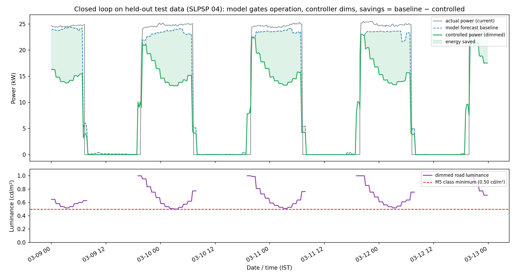
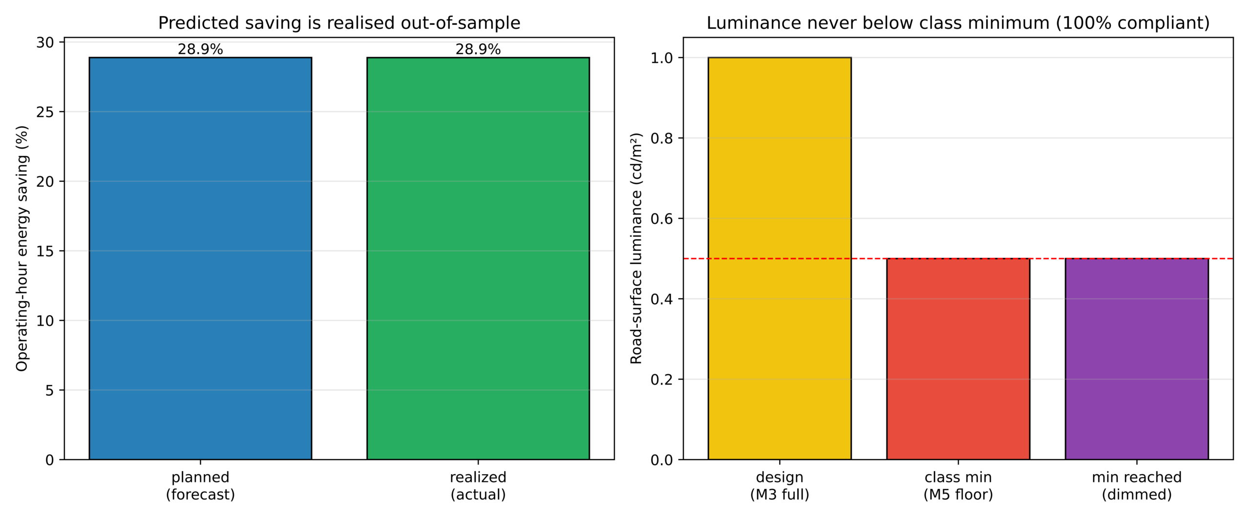
With the M3-to-M5 anchoring (a fifty-percent floor), the controller dims most in the empty small hours and holds full output during the evening traffic peak. During the held-out month, the simulated controller achieved an estimated operating-hour saving of approximately 28.9 percent while using the forecast baseline. Applying the same dimming policy to the actual metered power also gave 28.9 percent when rounded to one decimal place. This should not be interpreted as a perfect field performance, rather as a retrospective validation of the control policy. The mean luminosity during the operating hours is sixty-eight percent of the design output, that is, an average luminosity reduction of about thirty-two percent, reaching the fifty-percent floor in the deep night low-activity window. The luminance check is satisfied at every operating hour: the minimum realised road luminance is exactly 0.50 candela per square metre, which is equal to and never below the M5 class minimum, giving one-hundred-percent compliance. The Figures 3 and 4 show the closed loop over a representative four-day window and summarise the savings and luminance compliance.
Discussion
The added weather and traffic features do not materially sharpen point prediction; their value is that they make demand explainable from forecastable, controllable inputs, which is precisely what enables scheduling and control. The role of the model in the loop is to forecast the operating window and the demand baseline, so that a schedule and an expected savings can be computed in advance from the weather-and-traffic forecast, and to confirm, through an R-squared value of 0.895, that the conditions carry the demand signal that justifies the condition-driven control. The magnitude of the savings is set by the safety-bounded control policy, and the agreement between the planned and the realised savings shows that the operating window forecast is accurate enough that the plan is achievable.
Positioning against prior work, the present saving of about twenty-nine percent is lower than several other headline figures since it is bounded by an explicit luminance floor value computed conservatively with a fixed driver overhead that is validated out-of-sample and measured against the installation’s current constant-output behaviour rather than an idealised always-on baseline. The forty-eight to seventy percent range that is reported in large scale municipal implementations1 and the fifty five percent from the real-time hybrid control8 are achieved through further relaxation of the lighting class, or through direct sensing presence rather than through a more accurate demand model. Therefore, the contribution is methodological rigour and principled safety bounding rather than a claim to maximal savings.
The deployment challenges remain substantial: the controller assumes a typical traffic profile rather than real-time counts, a single weather location rather than on-pole sensing, and a linear power-to-output relationship. Plausible failure cases include the seasonally shifting dusk boundary, which a learned controller must track through solar radiation rather than through clock time; rare dense-fog events, which are often underrepresented in the data; and over-dimming if the floor value is set without reference to the road’s actual lighting class.
Limitations
The given dataset spans across four months of the cool, dry season only, therefore, monsoon and summer conditions, and a fully representative seasonal range, are unobserved, and the test month is a single seasonal slice. The traffic data input is a deterministic weekday-by-hour profile rather than real-time data; therefore, the controller is open-loop with respect to traffic. Weather is being drawn from a single grid point, with a thin tail of safety-relevant low-visibility events29,28. The savings are simulations that are validated against actual load, not a metered field deployment with physically dimmed lamps. For both localities, a single lighting class is considered, where a commercial and a residential street should occupy different light classes. The power-to-output model is a first-order linear approximation, and a mild residual overfitting remains.
Conclusion
A leakage-controlled, chronologically validated model is able to predict feeder-level streetlight power with an R-squared value of 0.895, using weather, traffic, and time alone, once the features that algebraically determine the target are removed. Adding weather and traffic data only improves the prediction modestly, and the apparently dominant solar-radiation feature is a daylight proxy rather than an independent signal, a result which is reported transparently rather than as an accuracy claim. The model’s value is realised in control: gating a luminance-anchored dimming policy, it supports a forecast-driven schedule that can reduce operating-hour power by about twenty-nine percent out-of-sample, validated against actual metered power and provably bounded by the M5 luminance minimum.
Thus, the objective of using a data model to reduce streetlight electricity through safe, condition-responsive dimming is demonstrated in simulation.
The principal next steps towards full validation are a metered field pilot with real-time traffic and on-pole light sensing, reinforcement-learning control that optimises against the demand forecast directly, and an edge implementation on the controllers. The broader implication is that honest, leakage-controlled modelling, coupled to a safety-bounded controller, can turn a familiar prediction task into a deployable, accountable energy-saving tool.
Code and data availability
The analysis code and processed dataset are available at https://github.com/adityakgoel/StreetLighting.git
Acknowledgments
The author would like to acknowledge an anonymous reviewer, whose detailed comments prompted the realisation of the leakage audit that completely reshaped the approach of this study and ended up substantially improving the analysis.
Appendix: Feature List and engineering rationale
The model uses contextual and temporal features only; all electrical channels were removed as leakage. Identifiers are one-hot encoded; time is cyclically encoded.
| Feature | Type / encoding | Rationale |
| Hour-of-day (sin, cos) | Cyclic | Captures the dominant day–night demand cycle without a 23→ 0 discontinuity. |
| Day-of-year (sin, cos) | Cyclic | Captures seasonal drift in dusk/dawn within the observed window. |
| Day-of-week; weekend flag | Integer / binary | Captures weekly activity patterns. |
| Solar radiation; sunshine duration | Numeric (weather) | Daylight proxies; strongly associated with on/off, though collinear with hour. |
| Temperature; relative humidity | Numeric (weather) | Tested for independent effect; found weak after time and radiation. |
| Rain; precipitation flag; cloud cover | Numeric / binary (weather) | Weather variation; low predictive value but retained for completeness and the fog rule. |
| Visibility | Numeric (weather) | Used by the controller’s safety overlay; negligible for power prediction. |
| Traffic congestion; monthly level | Numeric (traffic) | Activity proxy; collinear with time-of-day. |
| Controller identity; locality | One-hot | Captures per-feeder connected load and road type. |
References
- G. Pasolini, P. Toppan, A. Toppan, R. Bandiera, M. Mirabella, F. Zabini, D. Bonata, O. Andrisano. Comprehensive assessment of context-adaptive street lighting: technical aspects, economic insights, and measurements from large-scale, long-term implementations. Sensors. Vol. 24, pg. 5942, 2024, https://doi.org/10.3390/s24185942. [↩] [↩] [↩] [↩] [↩] [↩] [↩] [↩]
- I. Wojnicki, K. Komnata, L. Kotulski. Comparative study of road lighting efficiency in the context of CEN/TR 13201 2004 and 2014 lighting standards and dynamic control. Energies. Vol. 12, pg. 1524, 2019, https://doi.org/10.3390/en12081524. [↩] [↩] [↩] [↩] [↩] [↩]
- V. Krizanovic, K. Grgic, A. Pejkovic, D. Zagar. Energy savings in public lighting by using adaptive street lighting: a framework for energy-savings assessment and machine learning-based evaluation. Applied Sciences. Vol. 16, pg. 7917, 2026, https://doi.org/10.3390/app16167917. [↩] [↩] [↩] [↩]
- G. Gagliardi, M. Lupia, G. Cario, F. Tedesco, F. Cicchello Gaccio, F. Lo Scudo, A. Casavola. Advanced adaptive street lighting systems for smart cities. Smart Cities. Vol. 3, pg. 1495-1512, 2020, https://doi.org/10.3390/smartcities3040071. [↩] [↩] [↩]
- P. Mohandas, J. S. A. Dhanaraj, X.-Z. Gao. Artificial neural network based smart and energy efficient street lighting system: a case study for residential area in Hosur. Sustainable Cities and Society. Vol. 48, pg. 101499, 2019, https://doi.org/10.1016/j.scs.2019.101499. [↩] [↩] [↩]
- L. Valetti, G. Piccablotto, R. Taraglio, A. Pellegrino. Long-term monitoring campaign of LED street lighting systems: focus on photometric performances, maintenance and energy savings. Sustainability. Vol. 15, pg. 16910, 2023, https://doi.org/10.3390/su152416910. [↩] [↩]
- E. Belloni, C. Buratti, L. Lunghi, L. Martirano. A new street lighting control algorithm based on forecasted traffic data for electricity consumption reduction. Lighting Research & Technology. Vol. 56, pg. 481-501, 2024, https://doi.org/10.1177/14771535231194536. [↩] [↩] [↩] [↩]
- M. Takruri, K. P. Thulasingam, H. Attia, A. Omar, A. Altunaiji, S. Almaeeni. Design and implementation of a real-time street light dimming system based on a hybrid control architecture. International Journal of Distributed Sensor Networks. Vol. 2023, pg. 1-14, 2023, https://doi.org/10.1155/2023/6641563. [↩] [↩] [↩]
- X. Chen. The intelligent street light control system for preventing heavy fog of expressway based on ZigBee. Wireless Personal Communications. Vol. 121, pg. 353-359, 2021, https://doi.org/10.1007/s11277-021-08639-1. [↩]
- J. F. De Paz, J. Bajo, S. Rodriguez, G. Villarrubia, J. M. Corchado. Intelligent system for lighting control in smart cities. Information Sciences. Vol. 372, pg. 241-255, 2016, https://doi.org/10.1016/j.ins.2016.08.045. [↩] [↩] [↩]
- F. Sanchez-Sutil, A. Cano-Ortega. Smart regulation and efficiency energy system for street lighting with LoRa LPWAN. Sustainable Cities and Society. Vol. 70, pg. 102912, 2021, https://doi.org/10.1016/j.scs.2021.102912. [↩] [↩] [↩]
- P. Fang, M. Wang, J. Li, Q. Zhao, X. Zheng, H. Gao. A distributed intelligent lighting control system based on deep reinforcement learning. Applied Sciences. Vol. 13, pg. 9057, 2023, https://doi.org/10.3390/app13169057. [↩] [↩]
- H. I. Shaheen, B. Yang, Y. Zuo, M. Vasak, V. Lesic. Model predictive control for adaptive energy-efficient street lighting: a comprehensive framework and case study. IEEE Transactions on Industrial Electronics. Vol. 73, pg. 2960-2971, 2026, https://doi.org/10.1109/TIE.2025.3595989. [↩] [↩] [↩]
- A. Kumar, B. Yan, A. Bilton. Machine learning-based load forecasting for nanogrid peak load cost reduction. Energies. Vol. 15, pg. 6721, 2022, https://doi.org/10.3390/en15186721. [↩]
- G. Dudek. A comprehensive study of random forest for short-term load forecasting. Energies. Vol. 15, pg. 7547, 2022, https://doi.org/10.3390/en15207547. [↩] [↩] [↩]
- B. Magalhaes, P. Bento, J. Pombo, M. R. Calado, S. Mariano. Short-term load forecasting based on optimized random forest and optimal feature selection. Energies. Vol. 17, pg. 1926, 2024, https://doi.org/10.3390/en17081926. [↩] [↩]
- A. Chaianong, C. Winzer, M. Gellrich. Impacts of traffic data on short-term residential load forecasting before and during the COVID-19 pandemic. Energy Strategy Reviews. Vol. 43, pg. 100895, 2022, https://doi.org/10.1016/j.esr.2022.100895. [↩] [↩] [↩]
- Y. Hashimoto, Y. Ohashi, M. Nabeshima, Y. Shigeta, Y. Kikegawa, T. Ihara. Sensitivity of electricity consumption to air temperature, air humidity and solar radiation at the city-block scale in Osaka, Japan. Sustainable Cities and Society. Vol. 45, pg. 38-47, 2019, https://doi.org/10.1016/j.scs.2018.10.004. [↩] [↩]
- K. Chapagain, S. Kittipiyakul, P. Kulthanavit. Short-term electricity demand forecasting: impact analysis of temperature for Thailand. Energies. Vol. 13, pg. 2498, 2020, https://doi.org/10.3390/en13102498. [↩] [↩]
- P. Kumari, V. Garg, R. Kumar, K. Kumar. Impact of urban heat island formation on energy consumption in Delhi. Urban Climate. Vol. 36, pg. 100763, 2021, https://doi.org/10.1016/j.uclim.2020.100763. [↩]
- E. Wang, N. Alp. Identifying variable importance on mixed collinear building energy factor space by stochastic multi-statistic sensitivity analysis on TOPSIS with random decision forest. Energy. Vol. 329, pg. 136635, 2025, https://doi.org/10.1016/j.energy.2025.136635. [↩]
- M. Rotari, M. Kulahci. Variable selection wrapper in presence of correlated input variables for random forest models. Quality and Reliability Engineering International. Vol. 40, pg. 297-312, 2024, https://doi.org/10.1002/qre.3398. [↩]
- J. Song, Z. Zhang, G. Ren, J. Zhang, J. Ma. High-resolution traffic flow estimation for urban road network: incorporating traffic flow model into deep learning. Expert Systems with Applications. Vol. 302, pg. 130581, 2026, https://doi.org/10.1016/j.eswa.2025.130581. [↩]
- Y. Akashi, R. Ohashi, T. Uchida. The effect of luminance reduction on foveal task performance while implementing mesopic photometry in street lighting standards. Journal of Science and Technology in Lighting. Vol. 47, pg. 6-16, 2024, https://doi.org/10.2150/jstl.IEIJ220000656. [↩] [↩] [↩] [↩]
- I. Fryc, D. Czyzewski, J. Fan, C. D. Galatanu. The drive towards optimization of road lighting energy consumption based on mesopic vision – a suburban street case study. Energies. Vol. 14, pg. 1175, 2021, https://doi.org/10.3390/en14041175. [↩] [↩] [↩] [↩]
- R. Steinbach, C. Perkins, L. Tompson, S. Johnson, B. Armstrong, J. Green, C. Grundy, P. Wilkinson, P. Edwards. The effect of reduced street lighting on road casualties and crime in England and Wales: controlled interrupted time series analysis. Journal of Epidemiology and Community Health. Vol. 69, pg. 1118-1124, 2015, https://doi.org/10.1136/jech-2015-206012. [↩] [↩]
- Terra-Byte.ai. AI-powered operational intelligence (data platform). https://terra-byte.ai/ (accessed 17 September 2025). [↩]
- Open-Meteo. Historical Forecast API. https://open-meteo.com/en/docs/historical-forecast-api (accessed 14 June 2026). [↩] [↩]
- TomTom. New Delhi traffic report, TomTom Traffic Index. https://www.tomtom.com/traffic-index/city/new-delhi/ (accessed 14 June 2026). [↩] [↩]
- European Committee for Standardization. Road lighting – part 2: performance requirements (EN 13201-2:2015). See also CIE 115:2010, Lighting of roads for motor and pedestrian traffic. [↩]
- Bureau of Indian Standards. Code of practice for lighting of public thoroughfares (IS 1944); National Lighting Code (SP 72). [↩]