Improving Single-Engine Aircraft Safety Through Evolutionary Neural Networks

Abstract

Engine failure in a single-engine aircraft removes all thrust and leaves the pilot with one option: glide as far as possible while looking for a place to land. Standard practice is to hold a fixed best-glide speed taken from the aircraft handbook, but holding a constant target by hand is difficult, and earlier work has shown that the speed which loses the least altitude is not a single fixed number. This paper asks whether an automatic controller can glide further than a human holding that target, and whether a controller that learns its own inputs can do better than a conventional one. I built a Python simulator of a Cessna 152 that models forward motion, vertical motion and pitch, using Runge-Kutta integration and air density that varies with altitude. Its glide performance matches the handbook value of 1.6 NM per 1000 ft to within 0.4%. Three controllers were compared: human trials through a slider interface, a tuned PID controller holding a constant flight-path angle, and an evolutionary neural network whose weights were found by a genetic algorithm. The two automatic controllers were then tested across 400 combinations of starting altitude and airspeed, of which 390 were never seen during training. At the starting condition used for the human trials, the PID and neural controllers glided on average 17.03% and 17.77% further than the average human result. Across the 390 unseen conditions, the neural controller outperformed the PID by 35.73% on average. These results come from a two-dimensional simulator with no wind or turbulence, using one aircraft type, and the human comparison rests on trials by seven untrained participants through a simplified control interface.

Keywords: engine failure, glide distance, PID control, evolutionary neural network, flight simulation, general aviation

Introduction

As emerging AI technologies break barriers in many industries, I explored how they could be applied to improve a real world situation involving single-engine aircraft. Single engine aircraft carry multiple advantages over multi-engine aircraft such as being more fuel efficient, less expensive to maintain, and cheaper to purchase. However, all single-engine aircraft have a dangerous flaw: in the case of an engine failure, the aircraft will be left without thrust, and the best hope of survival is for the human pilot to maximize glide distance and find a possible location for landing. The ATSB reports a piston-engine failure rate of roughly 1 to 6 per 10,000 flight hours¹, and engine problems remain a recurring cause of general aviation accidents in the United States ².

To maximize flight distance, pilots are often told by the handbook or through the aforementioned guidance systems to obtain an optimal glide speed or optimal glide angle ³, and there are two major problems with this approach. First, there may not always be a single most optimal glide speed or glide angle during a thrustless descent due to varying air pressure, winds, and other external factors ⁴. Second, a human attempting to maintain a constant angle or speed is imperfect due to human errors and limitation on adjustment granularity and frequencies and, hence, results in loss of energy and glide distance.

Earlier work on this problem falls into three groups: certified avionics, optimizing the glide, and learned control.

Certified avionics. Some aircraft already carry systems that help after an engine failure. Loss of control in flight is one of the largest causes of fatal accidents across aviation ⁵. Garmin Smart Glide finds airports the aircraft can still reach. It checks terrain, obstacles and the current wind ^6,7, and it can tell the autopilot to hold best-glide speed ⁸. Garmin Autoland can fly a full approach and landing without pilot input ⁹. The Cirrus Airframe Parachute System takes a different approach and deploys a parachute ¹⁰. These systems help the pilot by primarily providing emergency guidance, autonomous landing, or parachute recovery. None of them tries to make the glide itself go further.

Optimizing the glide. Segal, Bar-Gill and Shimkin showed that the best glide speed is not one fixed number. It changes with the wind, and they derived what it should be ⁴. Irving covers the underlying theory of glide polars and speed-to-fly ¹¹. Other researchers have studied where a thrustless aircraft should glide, such as planning a route to a chosen landing site ¹², or finding the most energy-efficient path for a glider ¹³. The same group later extended their result to account for ground obstacles ¹⁴. Other methods build the glide path from stored flight manoeuvres ¹⁵, compute the full set of landing sites the aircraft can still reach ¹⁶, optimize the trajectory for an unmanned aircraft after engine failure ¹⁷, or plan the route with wind taken into account ¹⁸. The FAA’s glider handbook covers the same speed-to-fly ideas from a pilot’s point of view ¹⁹. All of this work calculates the answer from a known aerodynamic model. None of it learns a control policy.

Learned control. Neural networks have been used for flight control in many ways. Two recent reviews survey the field ^20,21. Reinforcement learning has been used to fly fixed-wing aircraft under model uncertainty ²², after actuator failures ²³, in changing wind ²⁴, and on high-performance aircraft ²⁵. One study tested a learned attitude controller in real flight rather than only in simulation ²⁶. Neuroevolution — using an evolutionary algorithm to find a network’s weights — has been applied to thrustless flight before. Stanley and Miikkulainen introduced NEAT, a widely used method ²⁷. Kim and Perez used NEAT to control a simulated aircraft while soaring ^28,29, and later added domain randomization to test how well the evolved controller handled conditions it had not trained on ³⁰. Gavra and van Kampen combined evolutionary search with reinforcement learning for flight control after a fault ³¹. These studies show that an evolved controller can fly a thrustless aircraft. However, their goal is to gain energy from wind, not to fly as far as possible on the energy the aircraft already has.

As far as I know, no one has directly compared these two approaches on the engine-out range problem. This paper does that. It compares a classical controller holding the handbook best-glide angle against an evolved neural controller that chooses its own elevator inputs, in one simulator checked against the Cessna 152 handbook, and tests both on starting conditions they were not tuned for.

To solve each of these problems, I investigated two approaches, one using a traditional feedback-based PID control system and the other using an evolutionary neural network (“ENN”) approach. The first, the PID controller, attempts to maintain a singular constant glide angle with significantly more accuracy than the human, solving the second problem but not the first. The second system, the ENN-based AI controller, is trained via a genetic algorithm to independently find any means to maximize distance, theoretically solving the first problem, and partially solving the second problem by having significantly greater accuracy than the human, but less than the PID controller

This paper asks three questions. First, can any controller glide further than one that simply holds the handbook best-glide ratio of 1.6 NM/1000ft? Second, if the evolved neural controller beats the PID controller, is the difference larger than the run-to-run variation caused by random starting weights and by the simulator’s time step? Third, does that advantage still hold at starting altitudes and speeds the network was never trained on?

The matching null hypotheses are that the handbook speed cannot be beaten, that the two controllers perform the same once run-to-run variation is accounted for, and that any advantage disappears on untrained conditions.

In the rest of this paper, I will discuss the physics model and simulator, the detailed design of each approach mentioned, the results and the conclusion.

Methods: Physics Model and Parameters

The simulator models the aircraft in two dimensions: forward motion, vertical motion, and pitch. A real aircraft has six degrees of freedom, but maximum glide range in still air is a longitudinal problem. Rolling, yawing and sideslip do not change how far the aircraft glides if it flies straight ahead, and at small bank angles they are only weakly coupled to the pitch axis. A reduced model also makes the comparison between controllers cleaner, because every controller has the same single input: the elevator. This choice has costs. The simulator cannot represent turning toward a landing site, crosswind, or a sideslip used to lose altitude. All of these matter in a real forced landing, and none of them are studied here.

To evaluate various approaches, I build a Python-based simulator with a multitude of considerations. First, I use a lot of specifications to make the plane similar to a Cessna 152 through online sources. I set the mass to 757kg ³, the wing area to 14.86m^2 3, the mean aerodynamic chord estimated as 1.47m through calculation

the moment of inertia approximated as 4067.5kgm^2 32, and the moment coefficient, coefficient of lift, and coefficient of drag at different angles approximated from the graphs available for the NACA 2412 airfoil ³³, the airfoil of the primary wing in the Cessna 152. These section coefficients follow the standard NACA airfoil data of Abbott and von Doenhoff ³⁴.

Second, to make the system dynamic, the density of air varies continuously as a function of altitude. Air density is computed as a function of altitude using the barometric formula, with sea-level pressure, temperature, and the temperature lapse rate taken from the U.S. Standard Atmosphere ³⁵.

The formula for air pressure at a given altitude h in meters is given by

where P₀ = 101,325 Pa as air pressure at sea level, L = 0.0065 K/m as the temperature lapse rate, T₀ = 288.15 K as temperature at sea level, g = 9.81 m/s² as gravity, M = 0.0289644 kg/mol as molar mass of air, and R = 8.31477 J/molK as the ideal gas constant.

Temperature at altitude follows the same lapse rate,

T = T₀ − Lh

and density follows from the ideal gas law,

ρ = PM/(RT)

where T is temperature in kelvin at altitude h, ρ is air density in kg/m³, and P, P₀, L, T₀, M and R are as defined above.

The exponent gM/(RL) evaluates to approximately 5.256 and is positive, so both pressure and density decrease with altitude. Table 1A compares the model’s output against the U.S. Standard Atmosphere at five altitudes spanning the range used in this study.

Altitude (m)	Simulated pressure (Pa)	Reference pressure (Pa)	Difference (%)	Simulated density (kg/m3)	Reference density (kg/m3)	Difference (%)
0	101,325.0	101,325.0	0.000	1.2250	1.2250	0.002
1,524	84,302.3	84,307.5	-0.006	1.0555	1.0555	-0.003
3,000	70,100.2	70,109.0	-0.013	0.9090	0.9091	-0.012
5,000	54,008.9	54,020.5	-0.021	0.7360	0.7361	-0.015
10,000	26,424.8	26,436.9	-0.046	0.4125	0.4127	-0.051

The model reproduces standard pressure and density to within 0.06% at every altitude tested.

Third, I ran the physics simulator using two methods. One takes in the current elevator input as well as the 6 state variables, which are velocity in the x axis, velocity in the y axis, position in the x axis, position in the y axis, current pitch relative to the horizon, and rate of change of pitch angle. It then returns the derivative of all of the state values, calculated from the previous state values as well as the elevator input. I calculate lift and drag directionally proportional to the aircraft using common formulas (using the dynamic air density), and parasite drag is included using a zero-lift drag coefficient. The zero-lift drag coefficient and the induced drag coefficient were mechanically calculated as 0.0440 and 0.0601 respectively to match the handbook’s best glide speed as 60 KIAS and best glide as 1.6 NM/1000ft. The functional coefficient of lift and drag respectively with state values as parameters are given by

where, C_L0 is the lift coefficient when the angle of attack is 0, estimated from NACA tables, C_Lα is the change in lift coefficient per radian change in angle of attack, α is angle of attack, C_D0 is the zero-lift drag coefficient, K is the induced drag coefficient, and C_L is the coefficient of lift.

The formula for force of lift and drag respectively with the state variables as parameters are given by

where ρ is the dynamic air density calculated by the above function, the lift coefficient and S are aforementioned constants, and V is the velocity of the aircraft, calculated from the velocity of its x and y components.

I estimated a stall function using the NACA2412 tables, and lift would collapse and drag would massively grow when the angle of attack exceeded 15 degrees. This hard boundary was selected instead of a curve as a simplified model because multiple curves exist at multiple different Reynold’s numbers. I then normalized the variables to earth-frame kinematics using trigonometry, and I divided the forces by mass to return accelerations. For torque, I multiplied the elevator angle input by an elevator effectiveness coefficient and added it to the rest of the values in the moment coefficient to simulate using the elevator, so a modified formula for pitching moment is used, given by

where C_M0 is the zero state pitching moment coefficient, C_Mα is the change in pitching moment coefficient per radian change of angle of attack, C_Mq is the pitch-damping rate derivative, c is the mean aerodynamic chord, C_E is a coefficient of elevator effectiveness, and ϵ is the current elevator angle. C_E is set to -1.1 per radian and was chosen to give an elevator authority consistent with a light general aviation aircraft rather than derived from Cessna 152 control surface geometry, and is a limitation of the model. Although this does not exactly physically represent elevator input, the result of the equation is effectively the same for the results of the experiment, since the elevator input must have varying effects as a function of air density, velocity squared, wing area, and chord as well. I then divide the pitching moment by the estimated moment of inertia to return angular acceleration.

In the second method, to update each state variable for each time step, dt, I chose the Runge-Kutta 4 (RK4) function. I prefer an RK4 method over Euler’s method because of the significant advantage in accuracy over extended periods of time, and standard practice in similar simulators ³⁶. The RK4 method uses the flight dynamics method described in the previous paragraph and returns the updated state values, effectively performing a step over a period of customizable time, dt. The formula for the RK4 function is given by

calculated from Simpson’s Rule, where

representing the exact slope of each state variable at the start of the step,

representing the estimated slope of each state variable at the midpoint of the step,

representing a more refined estimate of the slope of each state variable at the midpoint of the step, and

representing the estimated slope of each state variable at the end of the step, where X_n is a state variable, t is the current time, and f(a,b) is the respective function in the flight dynamics method.

The simulator is then run with parameters to sustain sufficient accuracy. Notably, dt is set to 0.01s, and the elevator input is a range between -10 degrees and 10 degrees. Although the actual Cessna 152 offers a range from -18 degrees to 25 degrees, this range is favored to simplify control and training for the human and the AI respectively.

Results

In this section, I discuss my results with human trials, PID controller and AI controller in detail.

Human Trials

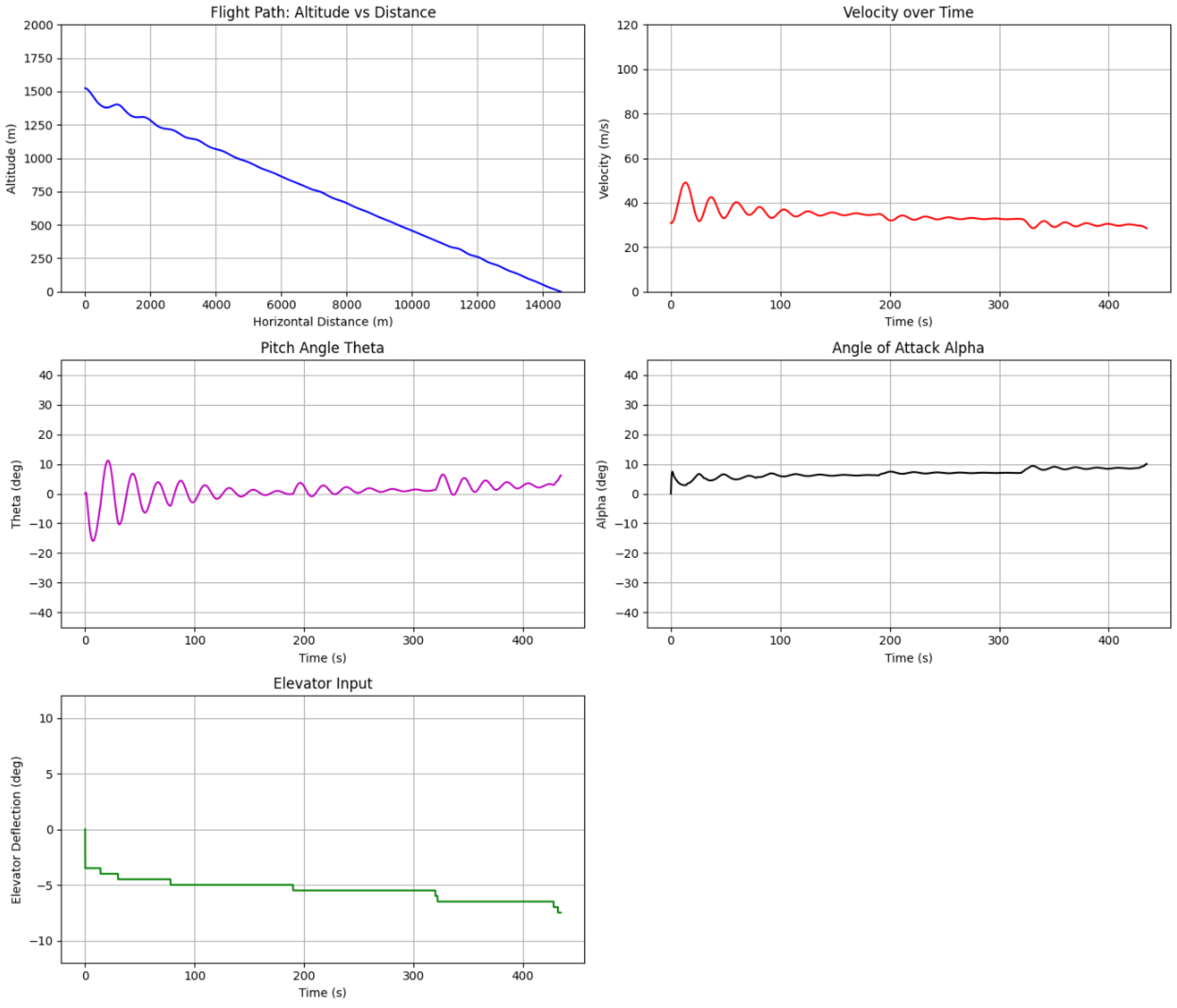
The human trials included seven persons who are not trained pilots but as my experiments compare with the handbook values and other references, these trials just serve as human trial examples. Each human would attempt 2 practice trials to understand the simulator before taking on multiple more trials to be included in the study. The participant with the least amount of trials had 10 trials, and the participant with the most amount of trials had 20 trials. The trials were performed at a starting state of 1524m (5000ft) and a starting velocity of 30.86m/s (60kts). These conditions were chosen as somewhat arbitrary values that maintained reasonable level flight and energy in testing. The human would have access to an ipywidget slider that would control the elevator from -10 degrees to 10 degrees. The simulator would then walk through 200 RK4 steps (2 seconds), while the human could change the elevator input during any step as the simulator ran, and update 5 graphs for the human to observe through matplotlib. These 5 graphs show position (displaying the path of the aircraft), velocity to time, pitch angle relative to horizon to time, angle of attack to time, and elevator input to time respectively.

Notably, it is hard for a human to control the simulator in finer-grained fashion since the human could realistically only receive and process new information every 2 seconds. As a result, with less fine tuned inputs, maintaining the optimal speed was significantly more difficult. The average distance among the 100 trials was roughly 10,961.4m and the greatest distance was 14,527.0m. In terms of NM travelled per 1000ft of altitude, the average rate was 1.362 NM/1000ft and the best rate was 1.568 NM/1000ft.

PID Controller and Trials

The Proportional-Integral-Derivative (PID) controller is designed to maintain a constant target glide angle for the aircraft. It does this by using the standard PID formula ^37,38 with coefficients chosen to optimize performance for the purpose of this paper, where the proportional term produces a directly proportional and antipodal input, the integral term softly accumulates past error to correct longstanding changes, and the derivative term reduces overshoot by predicting future outcomes.

The selected coefficients are chosen as 2.0 for proportional, 0.5 for integral, and 1.0 for derivative. The largest value is chosen for proportional, since the direct and instantaneous minute changes would be a large factor in maintaining a steady angle. The integral gain is kept small relative to the derivative gain. A large integral term can excite the aircraft’s phugoid mode, a slow oscillation in which altitude and airspeed trade against each other ³⁹. Hence, the formula for elevator input is approximately given by ϵ

where the integral and derivative terms are calculated as

at time t, where γ is the velocity vector to the horizon.

With these values, the PID controller has a similar initial state as the first set of the human trials at 1524 m and 30.87 m/s, with the only difference being initial orientation. Initially, the standard glide angle for the Cessna 152 is, calculated as:

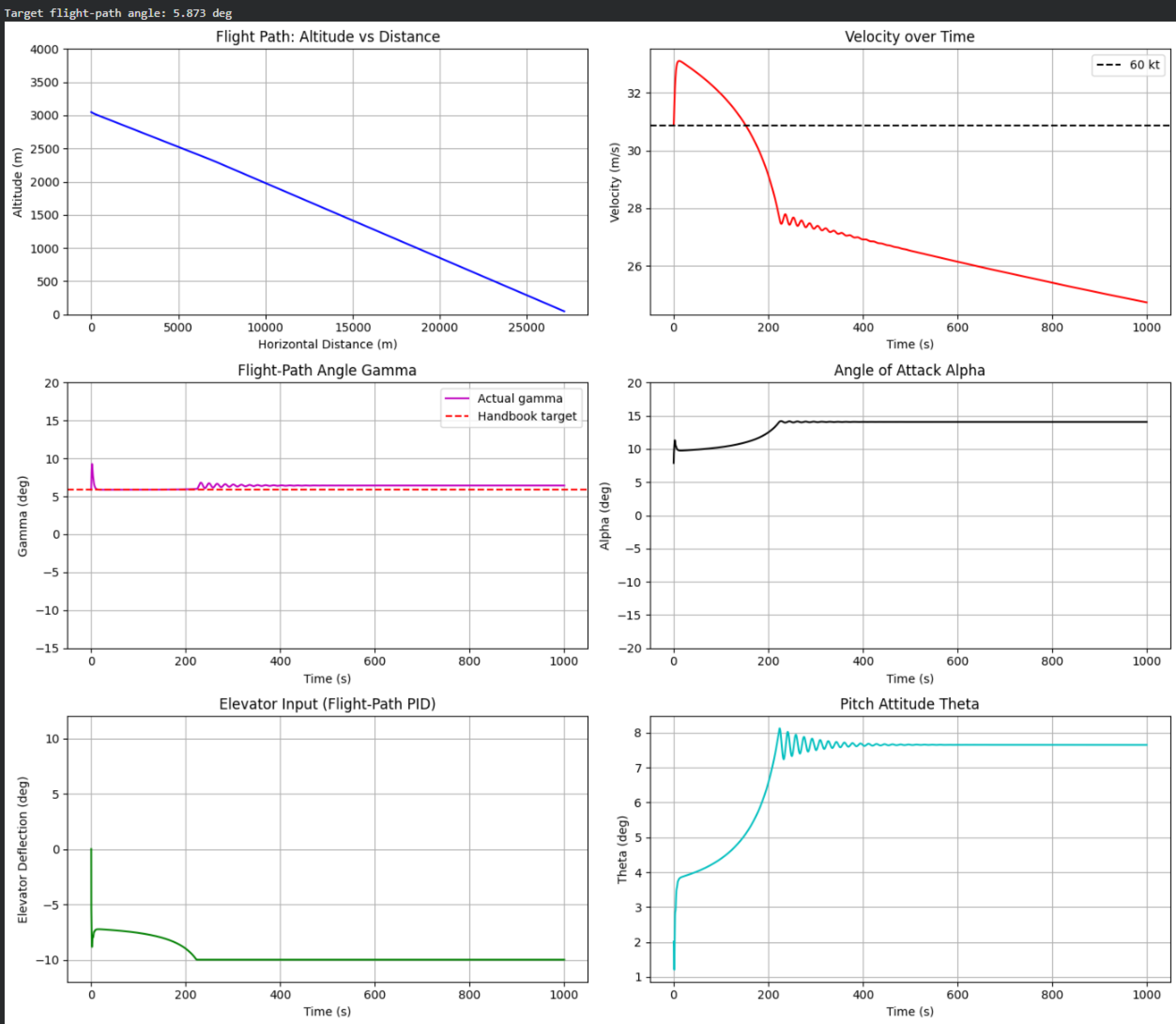
Hence, 5.873 degrees (since downwards is positive z) was chosen for the PID as a target angle, and the resulting distance was 14756.36m (7.97 NM) with a rate of 1.594 NM/1000ft, extremely similar to the handbook’s ideal 1.6 NM/1000ft.

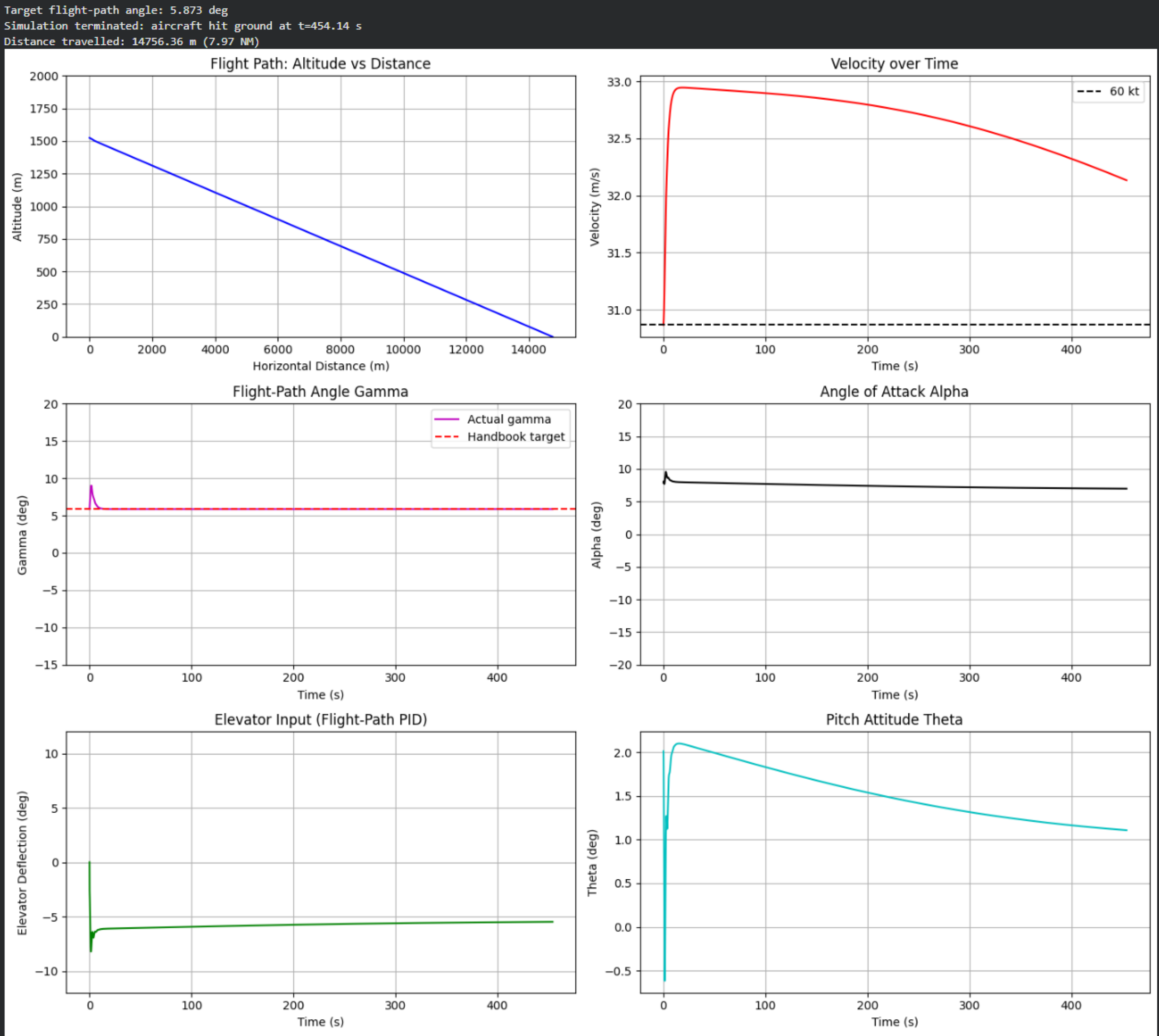
Besides a small adjustment period at the beginning of the glide, the PID is capable of maintaining the target angle stably and flies in a linear manner before touching down at a reasonable distance. This same PID controller was then placed in control of 400 different starting seeds ranging from 1000ft to 20000ft in increments of 1000ft and 40kts to 78kts TAS in increments of 2kts.

Controller	Mean (NM/1000ft)	Standard Deviation (NM/1000ft)	Min (NM/1000ft)	Max (NM/1000ft)	Median (NM/1000ft)
PID	1.176112	0.519264	0.267219	1.598080	1.474329

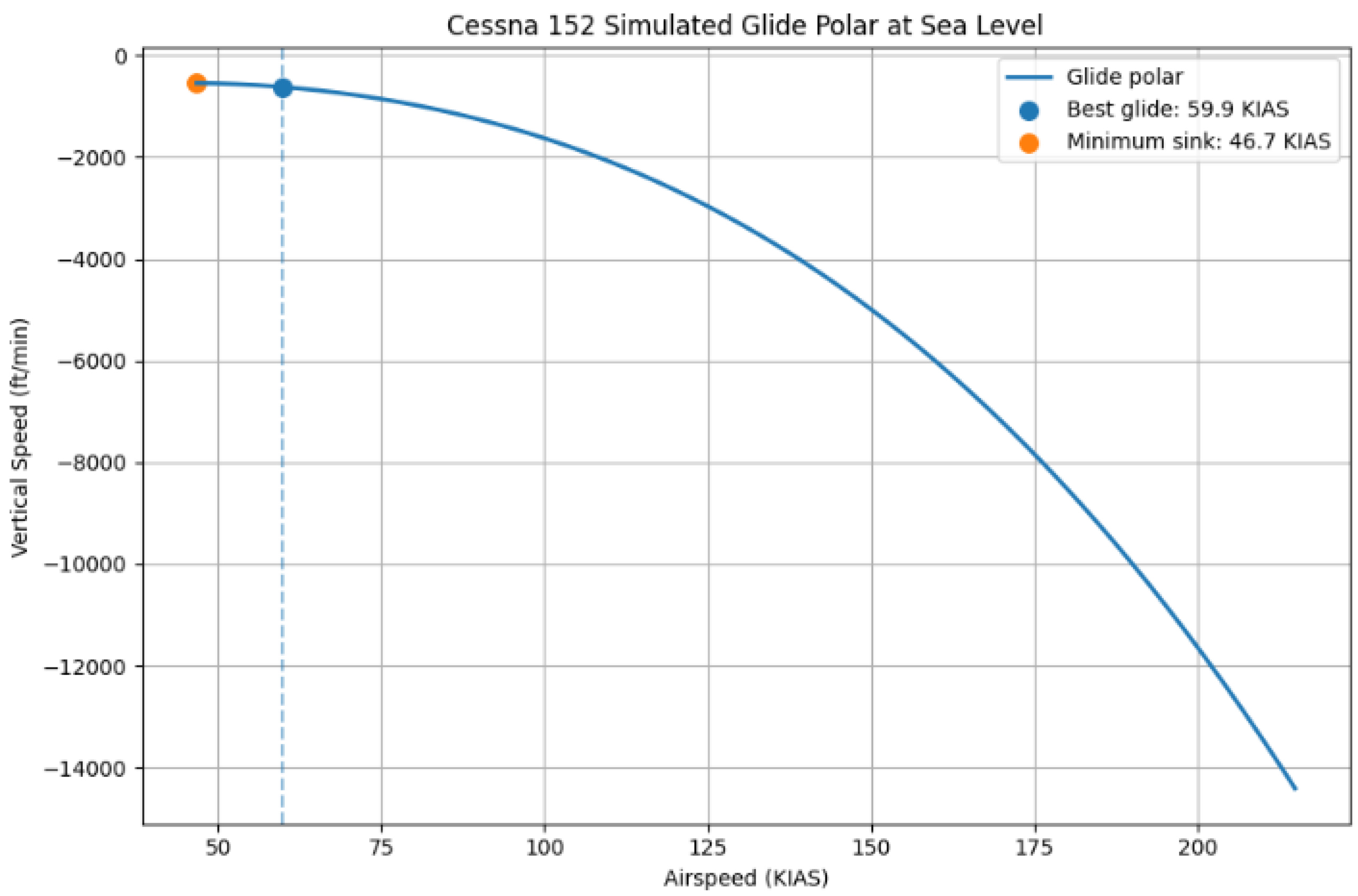
The Cessna 152 handbook gives a maximum glide performance of roughly 1.6 NM per 1000 ft with flaps up and the propeller windmilling. The PID controller reaches a maximum of 1.598 NM/1000 ft across all 400 starting conditions, and 1.594 NM/1000 ft at the 5000 ft, 60 kt case used for the human trials (Table 1B), both within 0.4% of the handbook figure. Figure 3B shows this across every starting condition: trials beginning above roughly 53 KIAS reach the benchmark, while slower starts fall short or enter a stall. Figure 3C plots the simulated glide polar at sea level, giving a best glide speed of 59.9 KIAS against the handbook value of 60 KIAS, a difference of 0.2%, and a minimum sink speed of 46.7 KIAS. These comparisons are a check on the simulator rather than on the controller, since the drag model, the density model and the integration scheme all feed into these numbers. Matching the published glide speed and glide performance indicates the aircraft model behaves like the real aircraft before any controller is compared. I do note that the agreement on overall glide performance does not by itself confirm that the individual drag components are correct, since errors in parasite and induced drag could offset one another but a careful implementation was made.

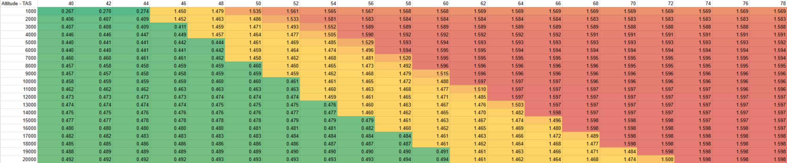
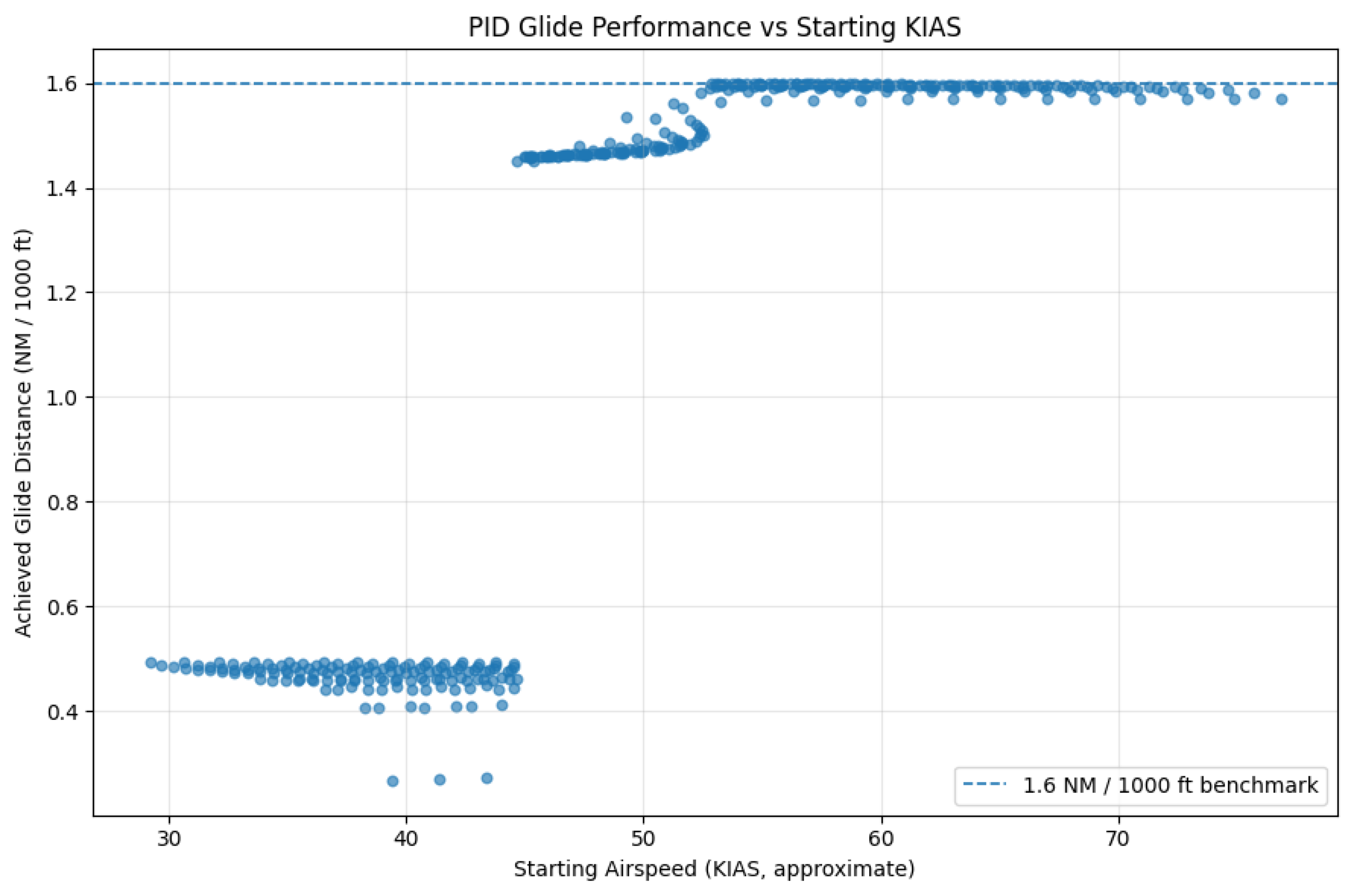
The PID performance is split into three regimes: the red regime represents cases where the PID controller was able to maintain a near-target angle for the duration of flight except a small adjustment period at the beginning; the yellow regime represents cases where after reaching a certain point, the aircraft did not have enough energy to maintain the target angle, and would travel slightly below that; the green regime represents cases where the PID entered a stall and lost massive amounts of energy.

AI Controller, Training, and Trials

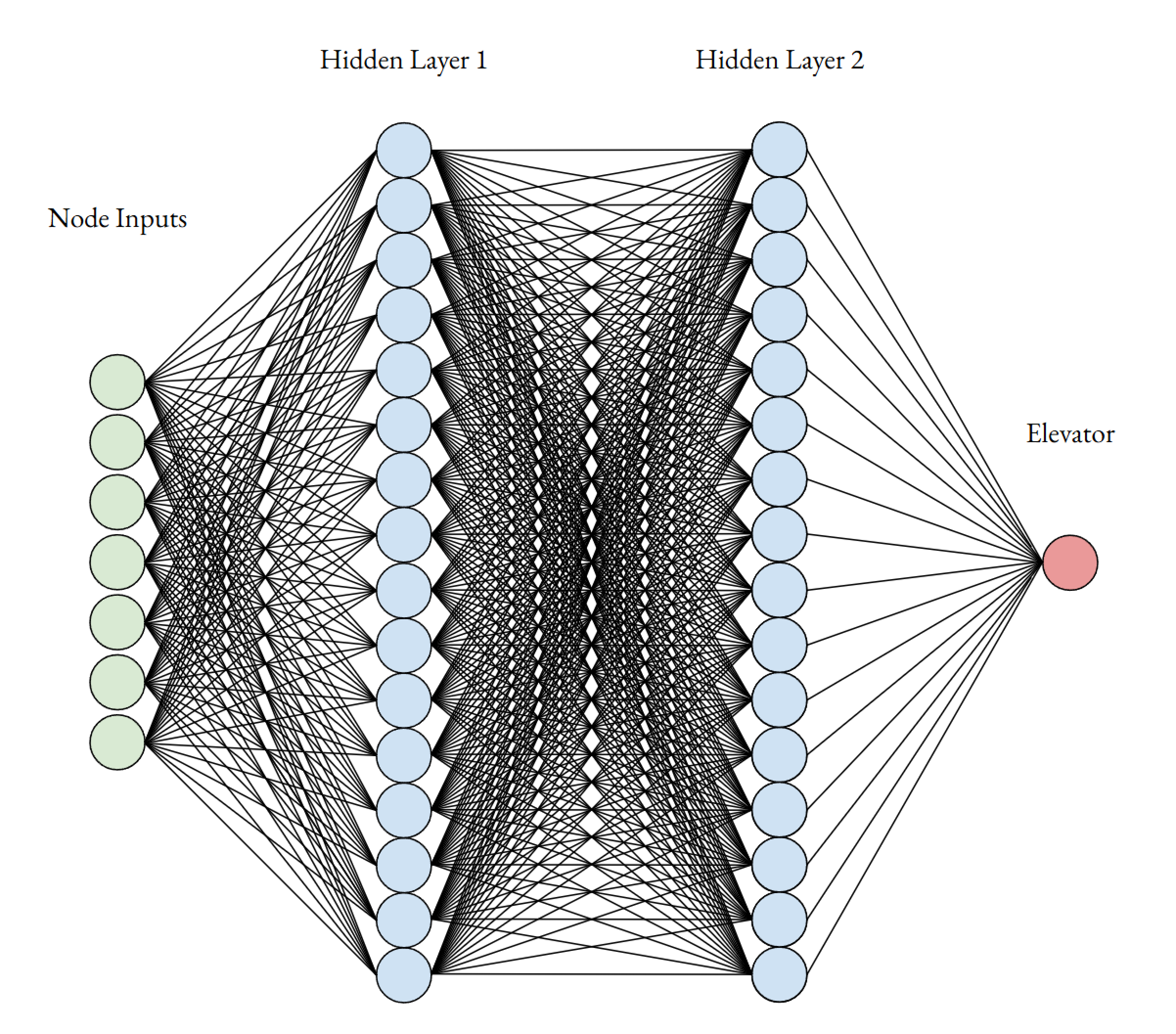
I further considered multiple different AI models to find a near-optimal distance and I chose an evolutionary neural network approach (the “ENN Approach”) to optimize the neural network’s weights in finding a glide distance better than earlier approaches ⁴⁰. The ENN approach uses all 6 state inputs and its update is governed by dt, which is set to 0.01 seconds for all experiments. In order to yield faster training, the 7 inputs are normalized first, given by the formulas,

where W_n is one of the node inputs and the state variables are horizontal distance, vertical distance, horizontal velocity, vertical velocity, pitch angle, angular velocity, and time step size, respectively.

After being normalized, the method takes the hyperbolic tangent of the weighted sum of each node input, given by,

and passes it into the 16 nodes of the first hidden layer, a set of 16 nodes that exist solely for mathematical computation to be passed into the next layer, where every letter a_n, …, g_n represents a different weight in the neural network. The hyperbolic tangent is chosen as it is a very common tool in these neural networks for approximating curves, as it delinearizes the network, and could have been used interchangeably with the sigmoid function, another typically used function.

The process then repeats for the next 16 nodes of the second hidden layer, given by

where, once again, every letter h_n, …, w_n represents a different weight in the neural network.

The final step returns an elevator input based on the 16 previous inputs, taking the hyperbolic tangent of the weighted sum and multiplying the value by 10, to increase the range from [-1, 1] to [-10, 10] to match the elevator ranges of the other control methods. This is given by the formula

Since I seek to maximize the distance travelled, I make the reward function in a one-way training with a genetic algorithm. This genetic algorithm approach is favored over traditional gradient-based methods because the goal is to optimize and find an excellent control system instead of matching an already known output dataset, which I showed in the previous section that a PID controller can do well.

For the first generation, 50 neural networks with random weights were generated, and each of them controlled the plane at 10 random starting seeds with altitudes ranging from 1000ft to 20000ft in increments of 1000ft and true airspeeds of 40 knots to 78 knots in increments of 2 knots. Only 10 out of 400 possible starting seeds were chosen in order to preserve sufficient unseen cases to test the ENN on later. Because the training and test conditions are drawn from the same grid, the 390 cases not used in training test how well a network interpolates across the operating envelope. Out of the 50 networks, the 10 networks with the greatest fitness, determined by mean NM travelled per 1000ft of altitude, were retained. These 10 elite networks would then move onto the next generation and create 40 new neural networks using the saved weights with slight modifications. Specifically, using a hyperparameter σ, which effectively served as a mutation standard deviation, the code would iterate through each weight in the parent’s network and gaussian perturbation with standard deviation σ is applied. The genetic algorithm would then train the ENN over 50 generations and freeze the weights of the final, fittest neural network.

This training process was performed 10 times with 10 different starting weights (or seeds) to ensure repeatability. The notation GA for genetic algorithms is used interchangeably with ENN.

Controller	Training Mean (NM/1000ft)	Testing Mean (NM/1000ft)	Testing Standard Deviation (NM/1000ft)
PID		1.176112	0.519264
GA 1000	1.592737	1.595023	0.047384
GA 1001	1.593035	1.596514	0.044922
GA 1002	1.593372	1.596131	0.047071
GA 1003	1.592302	1.595105	0.047521
GA 1004	1.591903	1.594700	0.047389
GA 1005	1.593136	1.594985	0.047612
GA 1006	1.600361	1.600340	0.030491
GA 1007	1.600649	1.599109	0.031311
GA 1008	1.593119	1.594471	0.071905
GA 1009	1.593722	1.597146	0.044667

The median network (GA 1003) was then further compared against the PID controller across all 400 starting positions in dt = 0.01. The mean difference between GA 1003 and the PID controller was 0.418922 NM/1000ft and the median paired difference between the two was 0.125206 NM/1000ft, roughly a 35.62% mean improvement and 10.73% median improvement over the PID controller. GA 1003 outperformed the PID in 399/400 cases, losing only at the starting seed 1000ft and 52kt TAS by 0.009507 NM/1000ft, a miniscule loss. GA 1003’s greatest victory over the PID controller was at the starting seed 1000ft and 44kt TAS, winning by 1.21579 NM/1000ft.

Parameter	Value
Network architecture
Input nodes	7 (6 state variables + timestep)
Hidden layers	2
Nodes per hidden layer	16
Output nodes	1 (elevator deflection)
Activation function	Hyperbolic tangent (tanh)
Total evolved weights	417
Topology	Fixed; weights only are evolved
Genetic algorithm
Population size	50
Elite networks retained	10
Offspring per generation	40
Selection method	Truncation on mean NM/1000 ft
Mutation	Gaussian perturbation, σ = 0.10
Crossover	None
Generations	50
Training conditions per individual	10
Independent training runs (seeds)	10
Simulation and fitness
Timestep, dt	0.01 s
Elevator deflection limits	−10° to +10°
Fitness function	Mean NM travelled per 1000 ft of altitude lost
Episode termination	Ground contact

Convergence Study

A timestep-convergence study was conducted to determine if the choice of using dt = 0.01 would significantly alter results. Hence, all 400 trials of both the PID controller and the median ENN controller GA 1003 were run in 4 different timesteps: 0.02, 0.01, 0.005, 0.002. The results of the larger 3 timesteps were then compared with the smallest timestep.

The ENN controller converges cleanly at every timestep, with maximum differences below 0.03%. The PID controller shows the same behaviour in most cases, but three of the 400 starting conditions cross the hard stall boundary at one timestep and not at another. Because a stall causes a large loss of energy, these three cases produce very large percentage differences that dominate the mean and maximum columns below in Table 3.

Timestep size (s)	Mean Difference	Median Difference	Max Difference
0.020	0.001904%	0.001000%	0.027342%
0.010	0.000918%	0.000466%	0.018812%
0.005	0.000436%	0.000192%	0.011651%
0.002	0%	0%	0%

Timestep size (s)	Mean Difference	Median Difference	Max Difference
0.02	1.0960%	0.001793%	228.740%
0.01	0.5773%	0.010180%	207.174%
0.005	0.001451%	0.000376%	0.033523%
0.002	0%	0%	0%

Excluding those three cases gives the following results in Table 5.

Timestep size (s)	Mean Difference	Median Difference	Max Difference
0.02	0.00533%	0.00177%	0.11892%
0.01	0.05949%	0.01016%	2.36821%
0.005	0.00145%	0.000376%	0.03352%
0.002	0%	0%	0%

One remaining case at dt = 0.01 differs by 2.37%, which is why the mean at that timestep exceeds the mean at dt = 0.02. This case sits close to the stall boundary without crossing it, so it was not excluded.

Across all 2397 comparisons for both controllers, only one differs from the finest timestep by more than 1.1%. These differences are far smaller than the 35.73% gap measured between the two controllers, so the choice of timestep does not affect the comparison, and the simulator is sufficiently convergent for the results reported here.

Discussion and Limitations

At the starting seed which the human trials were tested on, the human trial results have the lowest average rate 1.362 NM/1000ft. This is primarily due to the human inability to stably maintain the proper pitch angle through only the elevator input. Beyond the simulator and for future research, I conjecture that a trained pilot using a yoke instead of a widget slider to control the elevator would have significantly higher distances, but would not exceed the PID controller or AI controller on average.

Compared to the exact same starting seed, the PID controller results are notably successful, achieving a rate of 1.594 NM/1000ft at 5000ft and 60kts TAS. Due to the low computation required to calculate and adjust error, the PID controller would be excellent in real-time for implementation into aircraft. The PID controller could potentially be improved with different values K_P, K_I, and K_D, making the initial adjustment more energy efficient, and possibly increasing the distance. For future research, the PID controller may be more efficient with a different system that accommodates multiple glide angles at different sections of air density, or possibly a PID controller that follows a mechanically calculated ideal glide angle. I conjecture that such a sophisticated PID, while computationally more expensive, would significantly boost the performance of the PID.

Compared to the exact same starting seed, the ENN outperforms the human controller as well. Reaching the highest rate of the three controllers, the ENN achieved a rate of 1.604 NM/1000ft, bypassing the elusive 1.6 NM/1000ft rate which the PID aims to achieve.

Controller	Result at given seed (NM/1000ft)
Human	1.362
PID	1.594
GA 1003	1.604

Although the human dataset does not extend to the other 399 cases, a trained pilot in a real plane, following handbook statutes, would perform similarly to, but worse than, the PID, since the PID attempts to follow handbook statutes at a level of mechanical precision which a human could not achieve. Human deviation from the handbook may improve human results, but such a task is left to further research.

Beyond that single starting seed which the human cases were trialed on, over the 400 total possible starting configurations, the median ENN, GA 1003 outperforms the PID controller by 35.62% and wins 399/400 cases. This is primarily a result of two factors. First, as observed in Figure 4, the PID often lacks the energy to achieve its target glide angle, resulting in energy loss and an unoptimized distance. The ENN’s ability to learn different situations and adjust for these scenarios provides a notable advantage in the yellow regime. Second, the ENN is capable of maintaining more optimal glide angles which the PID does not have access to. The PID always attempts to maintain a certain glide angle, but this glide angle is only an approximate optimal, and is only truly optimal at a specific air density. The ENN is capable of finding a new optimal that adjusts to varying air densities better, and hence, finding a more optimal glide path.

Across all 10 training seeds, in the 390 test cases, the ENNs outperformed the PID by an average of 0.420240 NM/1000ft or a 35.73% improvement. Using a one-sample t-test, p < 0.00001, and this result is statistically significant.

While this improvement requires significantly more computation, in a more practical setting, the training of the ENN only needs to be performed once before its weights can be frozen, implemented into an aircraft, with the only computational expense being hyperbolic tangents and arithmetic, similar to the computational cost of the PID controller. This claim is supported by the fact that each ENN was trained only on 10 different starting seeds before being tested on an expanded set of 400 different starting seeds. For future research, the AI could be trained for a significantly longer amount of time, with a lower σ value in order to fine-tune the evolutionary neural network further.

In order to reduce discrepancies with reality, further research could incorporate wind vectors, turbulence, updrafts, and many other external events which I would expect to benefit the ENN controller significantly more than the PID controller, since the ENN approach has a significant advantage in finding complex non-linear solutions.

Overall, the findings suggest that PID controllers and ENN controllers offer more efficient descents in maximizing distance travelled compared to the human controller. Importantly, in the specific seed tested, the PID and ENN controllers both outperform the human by 17.03% and 17.77% respectively. For emergency engine failures, the PID controller and pre-trained neural network both offer low computation, high efficiency solutions that, if implemented into aircraft, could help reduce human errors and fatigue in these high-stress scenarios.

Further, across a larger variety of scenarios, the findings suggest that the ENN controller offers significantly more efficient descents compared to the PID controller. Outperforming the PID on average by 35.73% across 390 starting conditions not used in the ENN training. These conditions span the same altitude and airspeed ranges as the training set, so this tests interpolation across the operating envelope rather than extrapolation beyond it. On that basis, I conclude that the ENN controller could offer a critical improvement to current technologies and warrants further research.

Returning to the three questions raised at the outset: the handbook glide ratio can be beaten, since the ENN exceeds the PID controller (which holds the handbook target) in 399 of 400 starting conditions. The difference between the two controllers is larger than the run-to-run variation in the experiment, since the timestep study found only one comparison in 2397 differing by more than 1.1%, while the ENN advantage across ten independent training seeds averages 35.73% at p < 0.00001. That advantage does hold on conditions the networks were never trained on, since the 35.73% figure comes from the 390 held-out cases rather than the ten used in training. All three null hypotheses are therefore rejected, with the caveat that the third result demonstrates interpolation across the operating envelope rather than extrapolation beyond it.

Data and Code Availability

All code and seeds are available at https://github.com/Lionel-Messi-10/cessna-152 under the GNU General Public License Version 3. The version used for this paper is tagged Cessna 152 Simulator v1.1. The PID and ENN controller results can be reproduced by running the scripts in the repository.

Limitations

The pitching-moment model does not explicitly represent the horizontal tail. Instead, static pitch stability and pitch-rate damping are approximated through the lumped coefficients. As a result, the simulator captures restoring and damping tendencies but does not reproduce the full longitudinal dynamics of a real Cessna 152. Because pitch dynamics influence angle of attack, control response, and stall entry, this simplification may affect glide behavior and therefore is an important limitation of the model. Explicitly modeling the horizontal tail and validating the resulting pitch response against aircraft data would be a valuable next step.

Human resources were limited, as trials, even though sped-up, took a nontrivial amount of time. This prevented further comparisons between human trials and artificial controller trials. Further human data across the other 399 starting seeds could be an important next step for research.

Acknowledgements

I thank Kyle Kennedy, my mentor, for providing valuable insights, discussions, and resources that strongly improved the depth and clarity of this research and my parents for supporting me with the Google Colab resources that are necessary to run thousands of simulations

References

1. Australian Transport Safety Bureau. Engine Failures and Malfunctions in Light Aeroplanes, 2009–2014. ATSB Transport Safety Report AR-2013-107, Mar. 2016, https://www.atsb.gov.au/media/5769864/ar-2013-107-final-report.pdf. [↩]
2. National Transportation Safety Board. “US Civil Aviation Accident Dashboard: 2008–2024.” NTSB Statistical Reviews, https://www.ntsb.gov/safety/StatisticalReviews/Pages/CivilAviationDashboard.aspx. Accessed 15 August 2026. [↩]
3. Cessna Aircraft Company. Pilot’s Operating Handbook and FAA Approved Airplane Flight Manual: Cessna Model 152. Cessna Aircraft Company, Wichita, Kansas, 1978. [↩] [↩] [↩]
4. Segal, Daniel, Aharon Bar-Gill, and Nahum Shimkin. “Max-Range Glide in Engine Cutoff Emergencies Under Severe Wind.” Journal of Guidance, Control, and Dynamics, vol. 42, no. 8, Aug. 2019, pp. 1822–1835. [↩] [↩]
5. Belcastro, Christine M., John V. Foster, Gautam H. Shah, Irene M. Gregory, David E. Cox, Dennis A. Crider, Loren Groff, Richard L. Newman, and David H. Klyde. “Aircraft Loss of Control Problem Analysis and Research Toward a Holistic Solution.” Journal of Guidance, Control, and Dynamics, vol. 40, no. 4, 2017, pp. 733–775. [↩]
6. Garmin International. GTN Xi Series Airplane Flight Manual Supplement, P/N 190-01007-C2 Rev. 5. Garmin Ltd., https://static.garmin.com/pumac/190-01007-c2_05.pdf. Accessed 15 August 2026. [↩]
7. Garmin International. GTN Xi Series Pilot’s Guide, P/N 190-02327-03 Rev. G. Garmin Ltd., 2025, https://static.garmin.com/pumac/190-02327-03_g.pdf. Accessed 15 August 2026. [↩]
8. Garmin International. GFC 600 Pilot’s Guide, P/N 190-01488-00 Rev. H. Garmin Ltd., Sept. 2021, https://static.garmin.com/pumac/190-01488-00_h.pdf. Accessed 15 August 2026. [↩]
9. Garmin International. “Autoland.” Garmin Autonomí, https://www.garmin.com/en-US/autonomi/autoland/. Accessed 15 August 2026. [↩]
10. Cirrus Aircraft. CAPS Syllabus — Pilot Edition. Cirrus Aircraft, March 2013, https://cirrusaircraft.com/wp-content/uploads/2014/12/CAPS_Syllabus_Pilot_Edition.pdf. Accessed 4 June 2026. [↩]
11. Irving, Frank. The Paths of Soaring Flight. Imperial College Press, 1999, pp. 17–32. [↩]
12. Atkins, Ella M., Igor A. Portillo, and Matthew J. Strube. “Emergency Flight Planning Applied to Total Loss of Thrust.” Journal of Aircraft, vol. 43, no. 4, July–Aug. 2006, pp. 1205–1216. [↩]
13. Wolek, Artur, Eugene M. Cliff, and Craig A. Woolsey. “Energy-Optimal Paths for a Glider with Speed and Load Factor Controls.” Journal of Guidance, Control, and Dynamics, vol. 39, no. 2, Feb. 2016, pp. 397–405. [↩]
14. Segal, Daniel, Aharon Bar-Gill, and Nahum Shimkin. “Altitude-Loss Optimal Glides in Engine Failure Emergencies — Accounting for Ground Obstacles and Wind.” arXiv:2304.06499 [eess.SY], 13 Apr. 2023. [↩]
15. Adler, A., Aharon Bar-Gill, and Nahum Shimkin. “Optimal Flight Paths for Engine-out Emergency Landing using Flight Primitives.” Proceedings of the 24th Chinese Control and Decision Conference (CCDC), Taiyuan, China, May 2012, pp. 2908–2915. [↩]
16. Akametalu, Anayo K., Claire J. Tomlin, and Mo Chen. “Reachability-Based Forced Landing System.” Journal of Guidance, Control, and Dynamics, vol. 41, no. 12, Dec. 2018, pp. 2529–2542. [↩]
17. Fang, Xiang, Neng Wan, Hamidreza Jafarnejadsani, Donglei Sun, Florian Holzapfel, and Naira Hovakimyan. “Emergency Landing Trajectory Optimization for Fixed-Wing UAV under Engine Failure.” AIAA SciTech Forum, San Diego, CA, Jan. 2019. [↩]
18. Paul, Sandeep, Frederick Hole, Alexandra Zytek, and Carlos A. Varela. “Wind-Aware Trajectory Planning for Fixed-Wing Aircraft in Loss of Thrust Emergencies.” IEEE/AIAA 37th Digital Avionics Systems Conference (DASC), London, 2018. [↩]
19. Federal Aviation Administration. Glider Flying Handbook, FAA-H-8083-13A. U.S. Department of Transportation, 2013, https://www.faa.gov/regulations_policies/handbooks_manuals/aviation/glider_handbook/. Accessed 3 June 2026. [↩]
20. Richter, David J., Ricardo A. Calix, and Kyungbaek Kim. “A Review of Reinforcement Learning for Fixed-Wing Aircraft Control Tasks.” IEEE Access, vol. 12, 2024, pp. 103026–103048. [↩]
21. Emami, Seyed Ali, Paolo Castaldi, and Afshin Banazadeh. “Neural Network-Based Flight Control Systems: Present and Future.” Annual Reviews in Control, vol. 53, 2022, pp. 97–137, https://doi.org/10.1016/j.arcontrol.2022.04.006. [↩]
22. Marquis, Dennis J., Blake Wilhelm, Devaprakash Muniraj, and Mazen Farhood. “Adversarial Reinforcement Learning for Robust Control of Fixed-Wing Aircraft under Model Uncertainty.” arXiv:2510.16650, 2025. [↩]
23. Marquis, Dennis J., and Mazen Farhood. “Hypernetwork-Conditioned Reinforcement Learning for Robust Control of Fixed-Wing Aircraft under Actuator Failures.” arXiv:2604.03392, 2026. [↩]
24. Olivares, David, Pierre Fournier, Pavan Vasishta, and Julien Marzat. “Model-Free Versus Model-Based Reinforcement Learning for Fixed-Wing UAV Attitude Control Under Varying Wind Conditions.” arXiv:2409.17896, 2024. [↩]
25. De Marco, Agostino, Paolo M. D’Onza, and Sabato Manfredi. “A Deep Reinforcement Learning Control Approach for High-Performance Aircraft.” Nonlinear Dynamics, vol. 111, 2023, pp. 17037–17077, https://doi.org/10.1007/s11071-023-08725-y. [↩]
26. Bøhn, Eivind, Erlend M. Coates, Dirk Reinhardt, and Tor Arne Johansen. “Data-Efficient Deep Reinforcement Learning for Attitude Control of Fixed-Wing UAVs: Field Experiments.” IEEE Transactions on Neural Networks and Learning Systems, vol. 35, no. 3, 2024, pp. 3168–3180. [↩]
27. Stanley, Kenneth O., and Risto Miikkulainen. “Evolving Neural Networks Through Augmenting Topologies.” Evolutionary Computation, vol. 10, no. 2, 2002, pp. 99–127, https://doi.org/10.1162/106365602320169811. [↩]
28. Kim, Eric J., and Ruben E. Perez. “Neuroevolutionary Control for Autonomous Soaring.” Aerospace, vol. 8, no. 9, 2021, article 267, https://doi.org/10.3390/aerospace8090267. [↩]
29. Perez, Ruben E., Jonathan Arnal, and Peter W. Jansen. “Neuro-Evolutionary Control for Optimal Dynamic Soaring.” AIAA SciTech 2020 Forum, AIAA Paper 2020-1946, 2020, https://doi.org/10.2514/6.2020-1946. [↩]
30. Kim, Eric J., and Ruben E. Perez. “Robust Neurocontrol for Autonomous Dynamic Soaring.” Journal of Guidance, Control, and Dynamics, vol. 46, no. 5, 2023, pp. 924–938, https://doi.org/10.2514/1.G006803. [↩]
31. Gavra, Vlad, and Erik-Jan van Kampen. “Evolutionary Reinforcement Learning: Hybrid Approach for Safety-Informed Fault-Tolerant Flight Control.” Journal of Guidance, Control, and Dynamics, vol. 47, no. 5, 2024, pp. 887–900, https://doi.org/10.2514/1.G008112. [↩]
32. Krawczyk, Zack. “Evaluating Reduced-Order Urban Wind Models for Simulating Flight Dynamics of Advanced Aerial Mobility Aircraft.” Aerospace, vol. 11, no. 10, 2024, article 830, https://www.mdpi.com/2226-4310/11/10/830. Accessed 13 April 2026. [↩]
33. Airfoil Tools. “Polars for NACA 2412 (naca2412-il).” Airfoil Tools, http://airfoiltools.com/airfoil/details?airfoil=naca2412-il#polars. Accessed 13 April 2026. [↩]
34. Abbott, Ira H., and Albert E. von Doenhoff. Theory of Wing Sections: Including a Summary of Airfoil Data. Dover Publications, 1959. [↩]
35. National Oceanic and Atmospheric Administration, National Aeronautics and Space Administration, and United States Air Force. U.S. Standard Atmosphere, 1976. NOAA-S/T 76-1562, U.S. Government Printing Office, Washington DC, 1976. [↩] [↩]
36. Shah, Kamal, et al., editors. Qualitative and Computational Aspects of Dynamical Systems. IntechOpen, 2023. [↩]
37. Sudha, G., and S. N. Deepa. “Optimization for PID Control Parameters on Pitch Control of Aircraft Dynamics Based on Tuning Methods.” Applied Mathematics & Information Sciences, vol. 10, no. 1, 2016, pp. 343–350, https://doi.org/10.18576/amis/100136. [↩]
38. Åström, Karl J., and Tore Hägglund. PID Controllers: Theory, Design, and Tuning. 2nd ed., Instrument Society of America, 1995. [↩]
39. Vinh, Nguyen X. Flight Mechanics of High Performance Aircraft. Cambridge University Press, 1993. [↩]
40. Yao, Xin. “Evolving Artificial Neural Networks.” Proceedings of the IEEE, vol. 87, no. 9, Sept. 1999, pp. 1423–1447, https://doi.org/10.1109/5.784219. [↩]