Deciphering Ancient Nautical Charts: Precision Analysis of Zheng He’s Fleet Navigation System

Abstract

Six centuries ago, how did Zheng He’s fleet navigate across the open ocean? The Zheng He Nautical Chart records the Zhenlu–Qianxing (dead reckoning–celestial fix) navigation system. This study simulated the process of this system and conducted an analysis of its navigation performance on the route from Sumatra to Ceylon. A Monte Carlo simulation model was constructed using parameters such as sailing speed, the zhi-to-degree conversion ratio, and observation times recorded in historical documents. The impact of different parameters and error sources on navigation results was evaluated, and a sensitivity analysis was conducted on the navigation capabilities of Ming-era mariners. The results show that when the model uses parameters from historical records, the simulated routes remain within the middle and northern latitudes of Sri Lanka. Within archaeotechnology, the present modeling approach furnishes a quantitative lens on ancient Chinese navigation, showing its utility in studying fragmented historical records.

Keywords:​ Archaeotechnology, Computational Simulation, Ancient Navigation, Zheng He, Celestial Navigation

Introduction

The Zheng He Nautical Chart survives in the Ming military treatise Wubei Zhi. It is one of the most systematic records we have of how the Chinese navigated centuries ago^1,2. These records suggest that Zheng He’s fleets combined Zhenlu and Qianxing methods in navigation, linking dead reckoning with celestial fixes. This record indicates that Zheng He’s fleets employed a complex Zhenlu-Qianxing integrated navigation system —a practice of dead reckoning-celestial fix collaborative navigation³. This is a question: six hundred years ago, how did Zheng He’s fleet manage to succeed across the open ocean with this system?

As the pinnacle of ancient Chinese maritime technology, Zheng He’s voyages have been studied primarily along two lines of research.

One research direction focuses on historical and geographical studies based on textual analysis. These studies mainly involve the collation and modern annotation of place names in Zheng He’s Nautical Chart, in order to reconstruct the fleet’s routes and scope of activity. A representative study is Xiang Da’s annotated edition of the Liang Zhong Hai Dao Zhen Jing⁴. Current research in this field still focuses mainly on textual interpretation and qualitative description^5,6,7,8,9.

The second research direction focuses on the principles of ancient navigation techniques. These studies established the correspondence between the stars used in ancient Chinese navigation and their modern astronomical counterparts, such as Polaris and the Southern Cross. They also explained the usage and mathematical principles of tools such as the qianxingban(star altitude board) and the maritime compass, and provided possible meanings for observation units such as zhi and jiao^{10,11,12,13,14}. These studies analyze specific technical methods used in ancient navigation and provide the scientific foundation for research on ancient navigation.

Ancient maritime cultures around the world developed diverse navigation methods based on their own knowledge systems and environments. Polynesian voyagers relied largely on experiential knowledge, including memorizing star positions, reading wave patterns, and observing bird movements^15,16. Arab and Mediterranean sailors made extensive use of astronomical instruments such as the astrolabe, star tables and written navigation guides¹⁷. The Zheng He Nautical Chart provides both compass courses (zhenlu) and measurable stellar altitude records (qianxing). These records provide a basis for translating historical navigation practices into a computational model.

The existing historical records do not provide precise values for sailing speed, observation timing, or the conversion of zhi into angular measurements. Therefore, navigation simulations should not be based on a single fixed set of parameters. Instead of selecting one fixed historical route, this study examines how uncertain navigation parameters affected the navigation process through sensitivity analysis. By developing a Monte Carlo simulation model, this study quantifies how much error the system could tolerate and assesses its ability to maintain effective navigation without modern instruments. This simulation approach provides a quantitative perspective on ancient Chinese navigation and can also be extended to digital humanities research involving incomplete historical records.

Methods

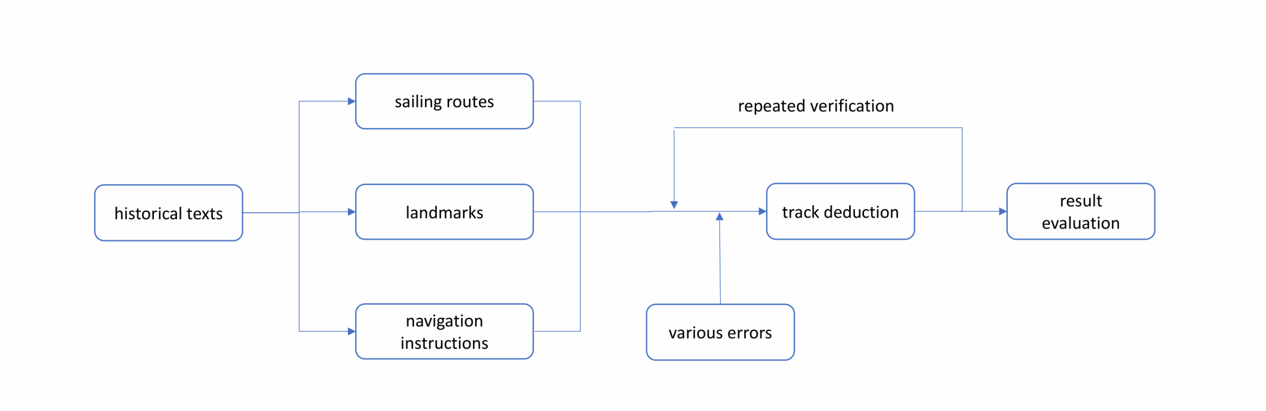
To answer the core question ” How exactly did Zheng He’s navigation system guide his fleet across the vast oceans?”, this study adopted a computer-based empirical approach to replay history. First, this study extracted sailing routes, landmarks, and stellar data from historical texts, translating them into input instructions for the simulation model. Second, it built a digital model that is capable of simulating the voyage and observation processes and incorporates realistic sources of error. Finally, the model was run automatically multiple times according to the instructions, and the results are analyzed to determine accuracy and stability (Figure 1).

Zheng He’s Nautical Chart and the Selection of the Simulated Route

The routes in the chart suggest different emphases in navigation methods between coastal and open-ocean sections. The coastal leg from Nanjing to Sumatra has many islands, so it mainly used Zhenlu (dead reckoning) for piloting. West of Sumatra, especially during the ocean-crossing legs across the Bay of Bengal and further into the Indian Ocean where land was distant and references scarce, Qianxing (celestial fix) were used extensively for positioning¹.

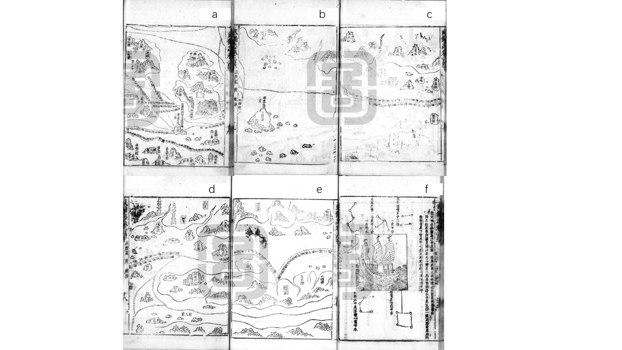
This paper focuses its simulation study on the more challenging trans-oceanic leg, selecting the “Sumatra to Ceylon” route as the simulation object (Figure 2). This choice is based on three main reasons: First, the record for this leg is very complete, containing both clear needle-course data and celestial-fix data. Second, it is representative; crossing the Bay of Bengal, it is a classic trans-oceanic segment that fully presents the challenges of open-ocean navigation. Third, it provides a more reliable basis for analysis: compared to other trans-oceanic legs, its needle-course directions are explicitly recorded, its distance (“geng”) records are consecutive, minimizing the uncertainty caused by ambiguous text or missing information.

Historical-Geographical Verification and Coordinate Determination of Key Landmarks

Accurate geographical coordinates are necessary to establish the simulation model. Building on traditional literature, this study also used simulation results as a reverse constraint to determine the coordinates of key landmarks on the “Sumatra to Ceylon” route¹⁸.

• Starting Point: Sumatra. The mainstream view was adopted⁶, placing it at the mouth of the Pase River in northern Sumatra.
• Key Point: Longxian Islet. The view that Longxian Islet corresponds to Pulau Rondo was adopted⁶.
• End Point: Ceylon. Candidate sites include Beirutala, Dondra Head, Galle, and Trincomalee in Sri Lanka⁶.

We summarize the conclusions and coordinates for these key landmarks in Table 1.

Parsing and Parameterization of Navigation Instructions

The core of this project’s simulation is converting historical records into a computable model. This section explains how this study parsed and parameterized the two main types of instructions in Zheng He’s Nautical Chart: needle courses and celestial fixes.

A needle course records a heading and distance. Directions use the Ming dynasty’s 24-point water compass system. The distance unit, “geng”, was converted into sailing time at a fixed speed based on related research. This study translated the original route descriptions into navigation commands (Table 1), such as converting “yòng qián xū zhēn shí’èr gēng” into a qián xū bearing held for twelve geng.

To verify the feasibility of the celestial observations and define the measurement benchmark, this study completed the following tasks:

Star Identification: Based on historical research, this study established a mapping between key ancient Chinese stars and their modern equivalents (e.g., Beichen corresponds to Polaris)¹⁸.

Astronomical Retro-calculation: Using the astronomy library Astropy, we retro-calculated the theoretical altitude of the target stars over the sailing area at local dawn on November 2, 1432 as the voyage’s start date.

The time for taking stellar altitudes isn’t clearly specified in historical records. Currently, scholars are divided into two schools of thought: one argues for observing when the target star reaches upper culmination to maximize precision; the other maintains the visibility of the sea horizon and advocates for observations during morning or evening twilight^3,19. The simulation adopts Yuan Qishu’s observation time of 06:00.

Determining Qianxing Parameters: Using astronomical calculations, this study found that in late November 1432, off the coast of Sri Lanka, it was impossible for all recorded stellar altitudes to satisfy the constraints of the Qianxing chart at a single moment. So the data logged by Zheng He’s fleet more likely came from observations taken at different times, not from a single instantaneous snapshot^20,21. The model assumes daily scheduled Qianxing observations. 

Polaris is selected as the celestial correction star, because it offers the most stable viewing conditions. Three conversion standards are used: 1.4°, 1.6°, and 1.8° per zhi^13,14,22,23.

To simulate the decision-making process of correcting course by the stars, this study set a threshold. This threshold determines whether a latitude correction is triggered. If the difference between the simulated theoretical star altitude and the recorded value exceeds the threshold, the deviation is deemed significant, and the fleet adjusts its course; else, the current course is not changed.

The threshold setting is based on the minimum readable resolution of the Qianxing board. The jiao is the smallest unit on qianxingban(star altitude board) and visual readings are subject to human limits, the max error for a single observation can be considered to be approximately 0.5 jiao (0.125 zhi). To avoid unnecessary adjustments caused by minor sea disturbances or slight reading tremors, the trigger threshold was set at 0.3 zhi. This maintains course stability and accuracy.

Based on the above, we created a set of celestial fix instructions for the “Sumatra to Ceylon” route (Table 1).

Category	Name	Set Value
Departure Time	Time	November 2, 1432 CE as the voyage start time
Route Waypoints	Start Point Coordinates	Sumatra: 5.1833°N, 96.4833°E
	Key Waypoint Coordinates	Longxian Islet: 6.0750°N, 95.1125°E
	End Point Coordinates	Ceylon: 8.5667°N, 81.2333°E
Celestial Data	Navigation Star Mapping	‘Beichen’: ‘Polaris’
	Star Coordinates	ICRS coordinates of stars
	Observation Time	Once per day at local dawn (approx. 06:00)
	Celestial fix correction threshold	Position is corrected (by sailing south or north) only when |theoretical star altitude − observed star altitude| > correction_threshold_zhi. 0.3zhi
Error Model	Systematic Error from Compass	A fixed value for the entire voyage, drawn,-2°、-1°、0°、+1°、+2° or N(0, 2.0°)
	Random Error from Steering	Independently generated for each step,N(0, 1°)、N(0, 2°)、N(0, 3°)、N(0, 4°)
	Random Error in Star Altitude Observation	Independently generated for each celestial observation,N(0, 0.05zhi)、N(0, 0.1zhi)、N(0, 0.15zhi)、N(0, 0.2zhi)
Navigation Instruction Parameters	Sailing Speed	2.9 km/h (i.e., sailing about 7 km per geng)
	Needle Course Parameters	Depart from Sumatra on a bearing of 307.5°, sail for twelve geng, then arrive and sail parallel to Longxian Islet. After passing Longxian Islet, begin the ocean crossing on a bearing of 285° for forty geng, then change course to 277.5° and continue for fifty geng; by this point, the fleet can sight Ceylon.
	Celestial Fix Parameters	Beichen (Polaris): three zhi and one jiao above the horizon

Simulation Model Construction for Zheng He’s Navigation System

This study built a modular simulation system to quantitatively assess the Zhenlu-Qianxing (dead reckoning-celestial fix) navigation system. We built a simulation system to model an ocean-going vessel following the instructions in Zheng He’s Nautical Chart, and tested its performance by adding realistic errors during the simulation.

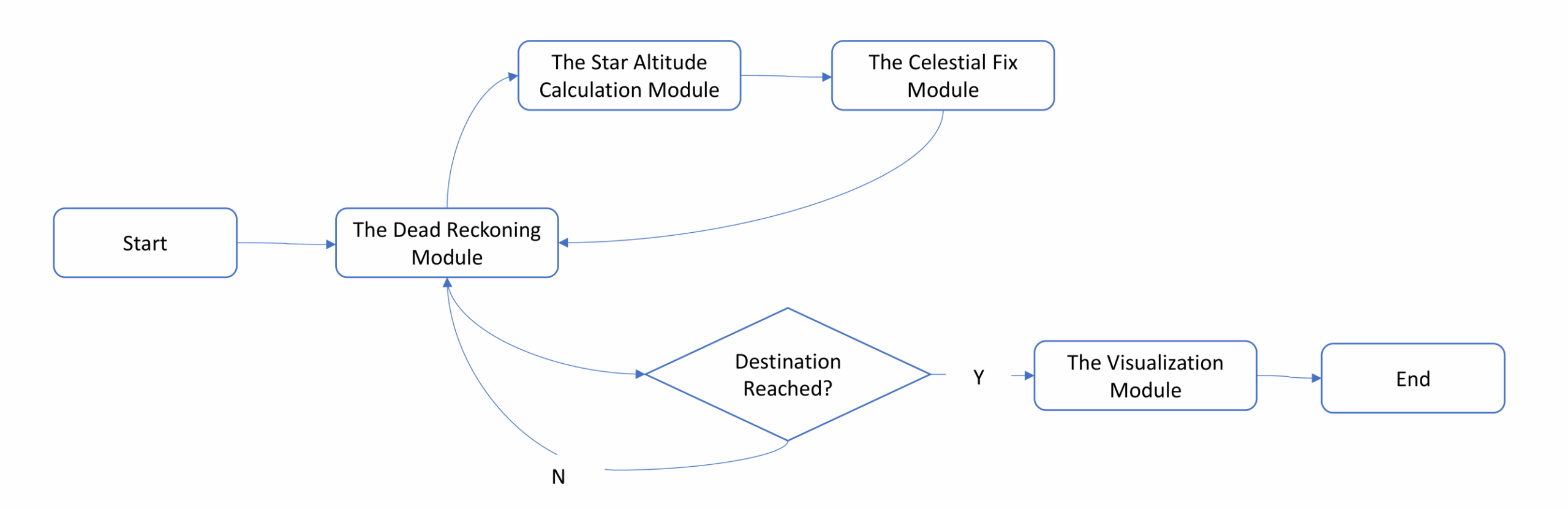
The core of the system is a predict-and-correct cycle (Figure 3): The dead reckoning module drives the ship based on instructions and an error model. The celestial fix module triggers at specific times, using astronomical observations to correct the ship’s position. The star altitude calculation module provides real-time theoretical astronomical data for the celestial fix module. The visualization module generates all trajectory plots and result charts. The program runs step-by-step in units of “geng” until it reaches the end condition (the ship reaching the easternmost longitude of Ceylon).

The main functional modules of the navigation system are the dead reckoning module, celestial fix module, star altitude calculation module, and visualization module. Additional control programs were built to manage the simulation workflow.

This module is the execution core of the navigation system, simulating real sailing that relies on compass and distance reckoning. Its input is the bearing and the distance. The module updates the ship’s position using a spherical dead reckoning algorithm with a given sailing speed. To simulate real sailing, a systematic compass error and a random steering error are introduced at each simulation step. During the voyage, the program checks if key turning points are reached or the current needle course segment is completed, and then automatically starts the next leg of the voyage. The simulated voyage is completed when the ship reaches the easternmost of Ceylon.

This module models the processes of celestial observation and positional correction. The procedure periodically uses astronomical observations to correct accumulated latitude errors from dead reckoning, keeping the route close to the target latitude. Daily observations are triggered at approximately 06:00 local time. Based on the theoretical altitude of Polaris calculated in real time, the module estimates the ship’s current latitude. The calculated theoretical latitude is then used by the program to simulate observation errors and obtain the actual observations made by the sailors. The estimated latitude is then compared to the target latitude specified in the navigation chart. If a deviation exists, the module calculates the direction and distance needed to turn onto a temporary corrective heading that will reduce this latitude difference. The ship follows the corrective heading until reaching the target latitude. It then returns to the original dead reckoning course.

This module calculates stellar coordinates in real-time based on the simulation time and ship position, implemented by calling the Astropy library. To ensure the accuracy of the astronomical retrocalculation, this study performed cross-validation. The altitude of the same star was calculated using Stellarium, and the difference was less than 2 arcseconds between the two methods.

This module plots the trajectory on a map based on real geographical data.

Simulation Experiment Design

For the “Sumatra to Ceylon” leg of Zheng He’s seventh voyage, we conducted the following three sets of experiments:

1. Core Parameter Sweep and Macro-Scale Trend Analysis: A baseline model was established to evaluate the effects of the sailing speed and the zhi-to-degree conversion ratio on the terminal location, excluding errors. Parameter Sweep: We tested four speed gradients (2.0 km/h, 2.5 km/h, 2.9 km/h, 3.5 km/h) and three zhi-conversion coefficients (1.4°, 1.6°, 1.8°). Macro-Scale Analysis: We tested all parameter sets and no errors were added. Results show where ships ended up near Sri Lanka. This can determine the system’s macro-sensitivity to key parameters.

2. Sensitivity Analysis of Navigational Error Sources: We used three independent sources of error and observed their disturbance to the baseline track: Compass Bias: We tested fixed offsets of -2°, -1°, 0°, +1°, and +2°. Test the effect of constant directional drift on the system. Steering Error: We tested σ of 1°, 2°, 3°, and 4°. These simulate human handling and rough seas. Astronomical Observation Error: We tested σ values of 0.05, 0.1, 0.15, and 0.2 zhi. Sensitivity Metrics: Rather than focusing on endpoint accuracy, this simulation analyzed how far the track deviated from the baseline and the rate of change in the scatter of endpoints.

3. Monte Carlo simulations of the final positions: To see how random errors affected where the ship ended up, we used Monte Carlo simulation. Simulation Setup: We used a sailing speed (2.9 km/h) and standard conversion rate (1.6°), and finished 1000 independent trials.  Errors: Compass (σ=2.0°), Steering (σ=1.5°), and Astronomical (σ=0.125 zhi). Statistical Analysis: Instead of just asking “Did it get there or not?”, we mapped all 1000 endpoints. Statistical analysis of the clustering of simulation results serves to assess the stability of the navigation system.

Results

Macro-Scale Performance Under Zero-Disturbance Conditions

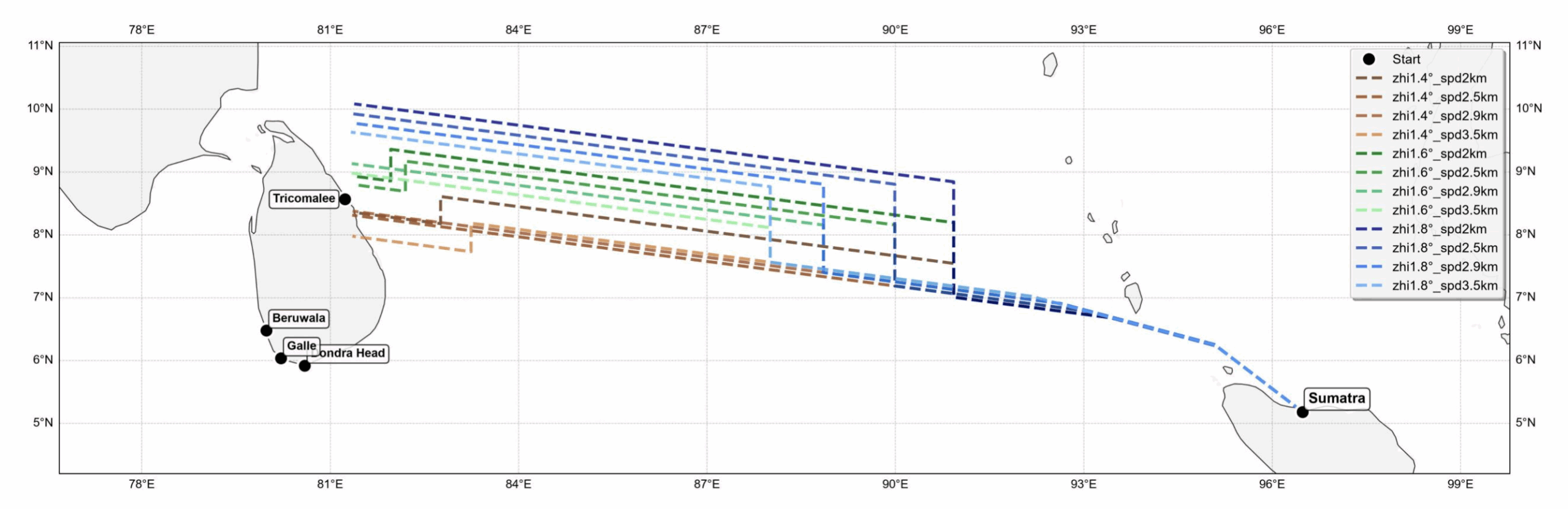
To test how sailing speed and the zhi-to-degree conversion rate affect the final outcome, we built a baseline model under ideal conditions. We tested all 12 combinations of four sailing speeds (2.0, 2.5, 2.9, and 3.5 km/h) and three conversion rates (1.4°, 1.6°, and 1.8°/zhi) (Figure 4, Table 2).

Zhi-to-Degree (°)​	Speed (km/h)​	Terminal Latitude (°)​	Arrival Time​	Mean Latitude (°)
1.4	2.0	8.36	1432-12-10	8.26
	2.5	8.31	1432-12-02
	2.9	8.38	1432-11-28
	3.5	7.98	1432-11-23
1.6	2.0	8.94	1432-12-10	8.96
	2.5	8.80	1432-12-02
	2.9	9.13	1432-11-28
	3.5	8.98	1432-11-23
1.8	2.0	10.08	1432-12-10	9.85
	2.5	9.93	1432-12-02
	2.9	9.77	1432-11-28
	3.5	9.63	1432-11-23

The simulation results show that changes in sailing speed caused only minor shifts in the final latitude, and it had a significant impact on sailing time. The zhi conversion rate was the dominant factor determining latitudinal drift. We find a larger conversion coefficient resulted in a higher final latitude. Importantly, although multiple parameter combinations were used, all endpoints were distributed within a narrow latitudinal band of 8.2°N to 10.1°N, this is the north-central part of the east coast of Sri Lanka. This tells us that, under ideal conditions, the Zhenlu–Qianxing (dead reckoning–celestial fix) system could reliably hold a vessel within a specific latitude corridor.

Trincomalee (approximately 8.5°N) falls within the core cluster. Other ports such as Beruwala, Dondra Head, and Galle fall outside this range. It suggests that this latitude band was the most probable target area under the simulated parameters. So, we think that the primary function of ancient Qianxing was to control north-south direction, rather than to locate a certain harbor.

Gong Zhen’s Xiyang Fanguo Zhi records: “…past this point, head west. After sailing seven to eight days, one sights Parrot’s Beak Mountain. After another two or three days, one sees Buddha Hall Mountain, arriving at the port of Ceylon called Bieluoli, where the ship anchors and lands”²⁴. Based on our findings, we offer the following interpretive inference: As the fleet approached Ceylon (Sri Lanka), they likely first sighted “Parrot’s Beak Mountain” (modern-day Trincomalee) and switched to visual piloting along the coast. They then sailed south along the east coast, rounded Buddha Hall Mountain, and finally arrived at Bieluoli.

Sensitivity Analysis of Error Sources

To isolate the effects of errors, we tested three independent noise sources against a baseline defined by a sailing speed of 2.9 km/h and a conversion rate of 1.6° per zhi.

Compass Bias

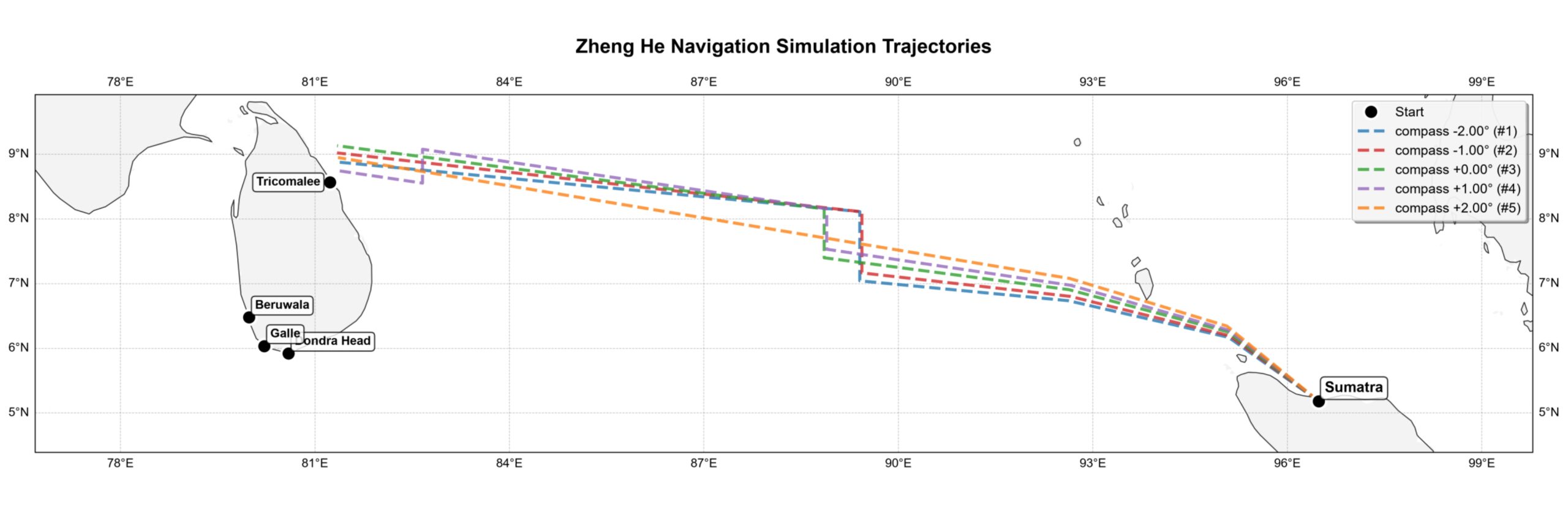
Compass Bias（°）	-2°	-1°	0°	+1°	+2°
Terminal Latitude (°)​	8.88	9.02	9.13	8.75	8.95
Latitudinal Deviation（°）	-0.25	-0.11	0	-0.38	-0.18
Latitudinal Deviation（km）	-27.5	-12.1	0	-41.8	-19.8

Data analysis shows that during the early stage of pure dead reckoning; a constant compass bias leads to an approximately linear drift in the track. However, once Qianxing correction is introduced, compass biases affect the timing and location of subsequent stellar observations. As a result, the final latitude deviation is not linearly related to the compass bias. The maximum observed offset was approximately 0.38° (about 42 km) (Figure 5, Table 3).

Steering Error 

Steering Error	N(0, 1°)	N(0, 2°)	N(0, 3°)	N(0, 4°)
Latitudinal Deviation（°）	-0.01	-0.03	-0.04	-0.05
Latitudinal Deviation（km）	-1.1	-3.3	-4.4	-5.5

Even with a large steering error (σ=4°), the latitude shift was only about 0.05° (roughly 5.5 km) (Table 4). This suggests that random steering error had limited influence on the transoceanic deviation.

Stellar Altitude Observation Error

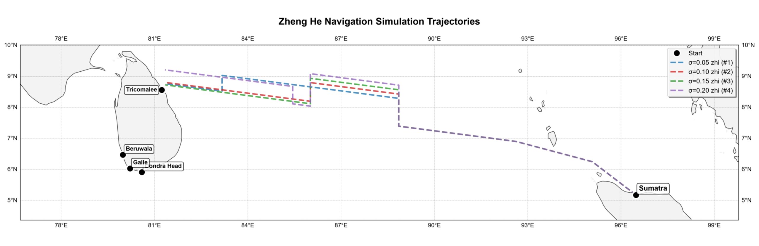
Stellar Altitude Observation Error	N (0, 0.05zhi)	N (0, 0.1zhi)	N (0, 0.15zhi)	N (0, 0.2zhi)
Latitudinal Deviation（°）	-0.36	-0.32	-0.4	0.09
Latitudinal Deviation (km)	-39.6	-35.2	-44	9.9

Before the first Qianxing correction, astronomical observation errors had a linear impact on route changes. However, as the voyage progressed, Qianxing corrections were repeatedly activated. Since the time and distance required for each course correction were different, no linear relationship was formed between astronomical observation errors and the final endpoint position (Figure 6, Table 5).

Statistical Characteristics and Robustness of Endpoint Distribution

This study conducted 1000 Monte Carlo simulations: compass bias N(0,2.0°), steering error σ=1.5°, and astronomical observation error σ=0.125zhi.

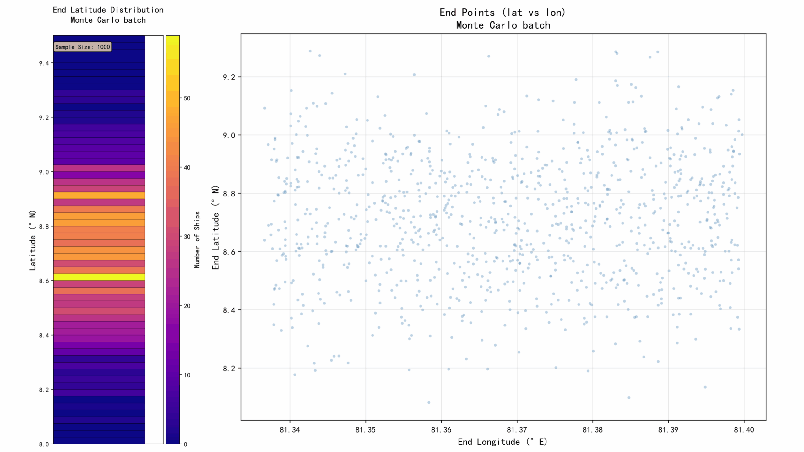
As shown in Figure 7, the latitude distribution of endpoints is a distinct single-peaked cluster. The peak interval of 8.4°N-8.8°N indicates that while the endpoints showed noticeable spread along the latitude axis, the majority landed along the northern coast of Sri Lanka.

Item	Mean	SD​	Median	(Q {25})	(Q {75})	95% CI Mean
Result	8.712°N	0.214°	8.715°N	8.566°N	8.863°N	[8.699°,8.725°] N

As shown in Table 6, the interquartile range (IQR) was 0.297° (approximately 33 km), encompassing 50% of all simulated endpoints. This proves that the fleet’s endpoints could maintain their position within a latitudinal band 30 km wide.

The results indicate that the system was capable of reliably holding the fleet at the appropriate latitude, even with different kinds of errors.

Discussion

The results show that although the observation tools used by Zheng He’s fleet had limited precision, the fleet relied on the Zhenlu-Qianxing cooperative system for navigation. The compass (zhenlu) provided high-frequency course guidance and star altitude measurements (qianxing) offered latitude corrections. Using both, the fleet was kept within a narrow band of latitudes.

Not all errors mattered equally. Random steering errors have little impact on the final endpoint position. While compass deviations and astronomical errors did introduce minor local course changes, the celestial correction mechanism kept these errors from snowballing into major divergence. The fact that the endpoints clustered together shows just how stable this navigation strategy really was.

The descriptions of zhenlu and qianxing were codified into parameterized simulation logic. This process accommodated ambiguities in the source material and evaluated the operational feasibility of the ancient navigation system.

The current scarcity of sources inevitably limited this study’s scope. Building on this work, we will examine how observation timing influences the endpoint and extends this analysis to navigation techniques across different languages and civilizations. Just as important, subsequent research demands a more integrated approach between historical geography and astronomy²⁵. It also requires adopting coastline data to perform a two-dimensional uncertainty analysis of the endpoints.

In summary, the purpose of this study is not to attempt to reconstruct the precise route of Zheng He’s fleet, but to use computer simulation to examine how this navigation system maintained positional control under uncertain conditions. The results show that this system could guide the fleet to the latitudinal region of Sri Lanka’s east coast without modern instruments. The approach and methods used in this study can also be applied to similar studies of ancient technological records.

References

1. Y.Y. Mao. Wubei Zhi [A Treatise on Armament Technology]. Zhongguo Guji Ziyuan Ku [China Ancient Books Resource Database], National Library of China. http://read.nlc.cn/allSearch/searchDetail?searchType=10024&showType=1&indexName=data_892&fid=411999032191 (Accessed 10 Feb. 2026). [↩] [↩]
2. Y.Z. Zhou. Explorations on Contrasts of Zheng He Hang Hai Tu Filed in Wu Bei Zhi and Nan Shu Zhi. Journal of Chinese Historical Geography, vol. 22, no. 2, pp. 145-152(2007). [↩]
3. Q.S. Yuan. A Study on the Ancient Star-sight Fixing. Navigation of China, no. 1, pp. 71–79 (1986). [↩] [↩]
4. D. Xiang. Liang Zhong Hai Dao Zhen Jing [Two Kinds of Rutters]. Zhonghua Book Company (1961). [↩]
5. N.W. Liu. A Tentative Investigation of Some Vernacular Names of Navigation Star. Journal of South China Normal College (Natural Science Edition), no. 1, pp. 15–20 (1982). [↩]
6. W.Q. Li. New Interpretation of Place Names and Route Analysis on the Recently Compiled Zheng He Nautical Chart. Journal of Dalian Marine College, vol. 11, pp. 123–131 (1985). [↩] [↩] [↩] [↩]
7. G.Q. Sun. A History of Ancient Chinese Navigation. Beijing: Ocean Press (2005). [↩]
8. N.W. Liu (ed.). Ancient Chinese Nautical Astronomy. Science Popularization Press Guangzhou Branch (1989). [↩]
9. C. Li. Research of the Genesis of the “Meridional Location of Navigation” Application in Ancient China. Journal of Chinese Historical Geography, vol. 29, no. 2, pp. 136–147(2014). [↩]
10. N.W. Liu. Interpretations of Hainan Fishers’ Genglubus. The Journal of South China Sea Studies, vol. 3, no. 1, pp. 22–26(2017). [↩]
11. W.Y. Pang. Introduction to Geographic Points and Navigation Points: And Head-on Pointers and Return Pointers in Genglubu. The Journal of South China Sea Studies, vol. 7, no. 3, pp. 59–66(2021). [↩]
12. Y.J. Liu. Interpretation of Needle Positions in the South China Sea Genglubu. Maritime History Studies, no. 1, pp. 15–23(2023). [↩]
13. D.Y. Wang. Research on Navigation Astronomy Technology Used by Zheng He’s Voyages (1405–1433). PhD diss., Jiangsu University of Science and Technology. https://doi.org/10.27171/d.cnki.ghdcc.2024.001494 (2024). [↩] [↩]
14. X.S. Chen. “Celestial Ruler” and Kamal: A Note on the Navigation Instruments of Ancient China and the Arabs. Studies in the History of Natural Sciences, vol. 37, pp. 139–155 (2018). [↩] [↩]
15. Á. Montenegro. Using Seafaring Simulations and Shortest-Hop Trajectories to Model the Prehistoric Colonization of Remote Oceania. Proceedings of the National Academy of Sciences, vol. 113, pp. 12685–12690 (2016). https://doi.org/10.1073/pnas.1612426113 [↩]
16. B.R. Finney. Pacific Navigation and Voyaging. The Polynesian Society (1976) [↩]
17. R. Pflederer. Portolan Charts: Vital Tool of the Age of Discovery. History Today, vol. 52, no. 5, May 2002, pp. 20–22 (2002). [↩]
18. K. Qiu. A Tentative Review of the Toponymic Research on Zheng He Hang Hai Tu — Also on Gu Jin Dui Zhao Zheng He Hang Hai Tu. Journal of Shanghai University (Social Sciences Edition), no. 2, pp. 56–63(1985). [↩] [↩]
19. J. Ren, et al. A Review of Research on the “Cross-Star” Celestial Navigation Technique. Maritime History Studies, no. 1, pp. 21–35(2022). [↩]
20. S.I. Hsu, et al. Use of Polaris and Vega to Position the Ships in Zheng-He’s Astronomical Navigation Charts. Journal of the Chinese Society for the History of Science and Technology, no. 24, December 2019, pp. 77–88 (2019). [↩]
21. N.L. Wang. Revisit Astro Navigation in Zheng He Era through Star Position Computation and Star Gazing. Journal of the Chinese Society for the History of Science and Technology, no. 27, December 2022, pp. 42–54 (2022). [↩]
22. N.W. Liu. A Nautical Chart Recording the Navigation Astronomy Technology Used by Zheng He’s Travelling. Scientia Geographica Sinica, vol. 25, pp. 748–753 (2005). https://doi.org/10.13249/j.cnki.sgs.2005.06.017 [↩]
23. J.Q. Zhang. Research on Zheng He’s Astronomical Navigation Technology. Geomatics World, vol. 15, pp. 86–96 (2017). [↩]
24. Z. Gong (Ming Dynasty). Xiyang Fanguo Zhi. Zhonghua Book Company (1961). [↩]
25. S.I. Hsu. Rambling on the New and Old Claims of Zheng-he’s Voyages in the Indian Ocean. Journal of Geographical Research, no. 43, pp. 21–41(2005). [↩]