Abstract
Proteins control nearly all biological processes, making them the primary target for therapeutic treatment. Drug development is concerned with optimizing the binding affinity between drugs (ligands) and target proteins, which involves predicting binding strength between novel protein-ligand pairs; however, the traditional method of conducting physical laboratory experiments to determine binding affinity is laborious and time-consuming, inhibiting the drug discovery process. Thus, groups of researchers have sought to leverage machine learning models to more efficiently predict binding, accelerating the identification of effective therapeutics. In this study, we tested various deep-learning based models, utilizing the molecular SMILES data of ligands to predict binding to 3 target proteins: BRD4, HSA, and sEH. We propose a hybrid GNNTransformer framework, which incorporates a multi-head attention mechanism and diverse molecular representations, including molecular fingerprints (ECFPs), metadata, and graph representation to achieve strong predictive performance. On all 3 proteins, the model improved accuracy, precision, recall, AUC, and f1_score from 50% to 70-80% and Average Precision to 70%. The success of this novel deep learning method on 3 structurally diverse proteins underscores the promise of multi-representational deep learning in the efficacy of drug discovery.
Keywords: Binding Affinity, Machine Learning, Proteins, Ligands, Drug-discovery, Deep Learning, Graph Neural Network, Transformer, Classification
Introduction
Proteins play a crucial role in biological processes, performing roles such as the transportation of materials, body acid-base balance, and catalysis. As such, the early stages of the drug discovery process involve finding molecular compounds that bind to certain target proteins to change their behavior/function. Throughout most of the history of modern therapeutics, drug molecules have been organic, small-molecule ligands. Recently, small molecules are even progressing in their potential for active cancer targeting, which previously only involved macromoleulces1.
The task of predicting the interactions between ligands and proteins is the core of drug discovery2. Binding affinity is a pivotal indicator of how strongly a potential drug molecule interacts with a target protein, which makes the prediction process vital for drug development3. The traditional methods of employing molecular dynamics and docking simulations to determine binding affinity are limited by their computational complexity and the lack of 3D protein structures available4. Furthermore, various experimental methods including isothermal titration calorimetry5 and surface plasmon resonance 6 prove costly and time-consuming. Thus, attention has been directed toward more efficient machine learning methods. Events such as the COVID-19 Pandemic have only revealed the urgent need for potent computational methods of drug development. To put into perspective, the FDA has approved of only 2,000 novel molecular entities. In contrast, the number of chemicals in drug-like space has been estimated to be 10^60, where effective treatments for human ailments are bound to be hiding7.
The ultimate question is: How can we leverage Machine Learning methods to best predict the binding affinities of ligands and target proteins with limited computational power and complexity?
To start, the dataset we utilized contained molecular SMILES data, which are linear representations of 3D molecules8, and binary binding affinity data for 3 proteins — BRD4, HSA, and sEH. Thus, our models would be supervised learning, classification-based algorithms. Many competing models deal with regression (e.g. DeepDTA, MDeePred, GraphDTA), which rely on precise binding affinity values; however, these values also come with great experimental uncertainty and can vary greatly across studies. Apart from reducing sensitivity to regression noise, classification allows our models to focus on broad distinctions between molecules and offers a more interpretable and actionable output for clinicians.
We started from traditional ML models, including Logistic Regression and K-Nearest Neighbors, operating solely on molecular fingerprints and metadata to assess the baseline ability for global molecular descriptors to capture and predict binding affinity. Although these simple, traditional ML models possess low computational cost, their predicting ability is limited due to oversimplification. Protein-ligand binding is a complex process that involves complex feature extraction and representation. On the other hand, deep learning ML can automatically extract advanced features from raw data and perform feature representation. In regards to the deep-learning models, we began with the 1-Dimensional Convolutional Neural Network (1D CNN), which took molecular SMILES data converted to molecular fingerprints (ECFPs) as its input representation. The 2-D CNN used pre-processed image representations of molecules. These CNNs were used to evaluate whether spatial or sequential analysis of molecular fingerprints would significantly enhance predictive power. Next, Graph Neural Networks (GNNs) were incorporated, converting molecular SMILES data to 2D graph representations to assess a focus on local dependencies and atom connectivities. Finally, the Transformer architecture used molecular sequence data (ECFPs) and involved a multi-head attention mechanism as well as relational modeling of the sequence data. We looked at the Transformer framework on its own to assess whether the capturing of long-range, non-localized feature relationships and contextual information proved advantageous over simple sequential, structural, or spatial patterns. The main model metrics we looked at were accuracy, precision, recall, f1_score, AUC, as well as average precision (specifically for comparison to competing methods).
Ultimately, we hypothesize that integrating diverse molecular representations within a hybrid GNN-Transformer framework will improve protein-ligand binding prediction compared to models using limited representation types.
Background
The two types of machine learning algorithms to predict protein-ligand binding affinity are interaction-free and interaction methods, and each has its benefits and drawbacks. Interaction-free methods largely involve deep learning models, and they succeed in that they aren’t limited to already-known protein-ligand complexes, can include long-range interactions between ligand and protein, and are not computationally expensive (Fig. 2). However, they often require a high homology of samples and lack the extraction of some chemical bond information. These methods can be categorized into sequenced-based models, graph-based models, and multimodal models. In this study we will specifically look at multimodal models like AttentionMGT-DTA, which employs two graph transformer modules to learn structural features of ligands and protein pockets while incorporating 1D sequence embeddings9. On the other hand, interaction-based methods, such as molecular docking simulations (Fig. 1) are able to improve generalization capability but are computationally expensive and lack long-range interactions10.
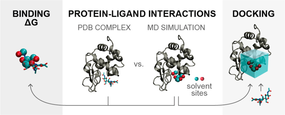
Published data by Arcon, et al., 201711.
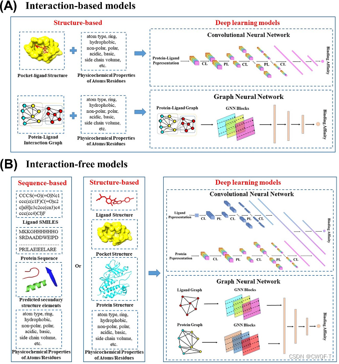
Figure 2 | Interaction-free deep learning model; Published data by Wang, et al., 2024
Numerous deep learning methods have been attempted, with varying results depending on the strategy and complexity of the approach. As a sequence-based model, DeepDTA uses only protein and ligand sequences, which are fed into 2 CNN blocks and a multi-layer perceptron (MLP). Similarly, GNNSeq relies solely on sequential features, performing hierarchical sequence learning through the integration of GNN, XGBoost, and Random Forest. This method eliminates the need for pre-docked complexes or high-quality structural data12.
Another competing method is DeepCDA, which combines the CNN with long short-term memory (LSTM) networks with a 2-sided attention mechanism13. DeepDTAF integrates local and global contextual features, which refer to the protein pocket (the localized area where the ligand binds to) and broader features respectively. The model utilizes dialed convolution to capture multiscale long-range interactions. However, it fell short of having a large enough training dataset to reduce reliance on training data types4.
Although sequence-based models can learn from contextual information in the sequence and are relatively mature in the field of representing proteins and ligands, they lack spatial infrmation14. Graph-based models overcome this disadvantage. GraphDTA, for instance, employs 2 graph neural network (GNN) blocks followed by fully connected layers to predict affinity13.
Previous methods encounter four main impediments which limit their capabilities for strong prediction and generalization. Primarily, previous deep-learning models struggle with low-quality databases that contain hundreds of ligands but only dozens of proteins and inaccurate or oversimplified input representations. In addition, models have difficulty with data imbalance (i.e. significantly more non-binding data samples compared to binding data samples), causing poor model performance10. Notably, past methods often only extract sequential information, losing vital spatial information or vice versa15. Lastly, predecessors of the binding issue lack the capturing of complex interactions between protein-ligand pairs such as electrostatic forces or hydrogen bonding10.
Methodology and Experimental Framework
Dataset Description
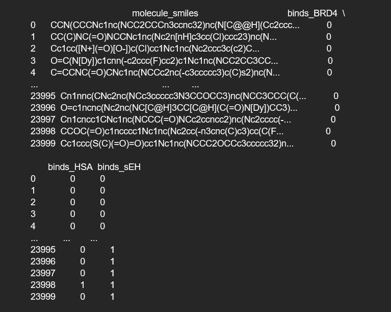
The kaggle competition host Leash Biosciences physically tested 133M small molecules for their ability to interact with one of three protein targets using DNA-encoded chemical library (DEL) technology. They created the dataset the Big Encoded Library for Chemical Assessment (BELKA).
In order to reduce computational cost through efficient storage, we used duckdb to directly read the parquet files and perform database connection. The entire dataset contains 7 columns, but only 4 relevant columns: 1 molecular_smiles column and 3 output columns corresponding to 3 different target proteins. The output columns classify if the compound binds to that protein or not. In the parquet datasets, we selected 12,000 data samples from each class (non-binding and binding) for my training, performing scaffold-based partitioning to ensure that all molecule structures are represented and prevent generalization. Similarly, we then selected 3,000 data samples at random from each class for our testing dataset., using the same stratified sampling technique. Thus, in total the training dataset contained 24,000 data samples, and the testing dataset contained 6,000 data samples (75% training, 25% testing), each evenly divided between classes. We split my training dataset into validation and training datasets (ratio = 0.2) stratified along the true output column to ensure equal numbers of each class.
Below is a snippet of my training dataset:
Model Development and Training Strategy
The general strategy to uncover the best-performing machine learning model was to start with simpler models and work towards more convoluted, computationally expensive models. To that end, we began experimenting with baseline models such as Logistic Regression, Random Forest, and Decision Tree Classification to set a performance floor. Logistic Regression tested for linear separability in the chemical space; in other words, it tested whether the difference between a protein-binder and a non-binder is determined by specific features only. Meanwhile, Random Forests/Decision Trees tested if non-linear decision boundaries were sufficient for classification. However, these baseline models were essentially coin tosses, so we determined that binding activity is not likely determined by the simple presence or absence of chemical fragments. We then began experimenting with 1-D and 2-D Convolutional Neural Networks to experiment with spatial and local feature extraction, utilizing different input representations — namely Extended Connectivity Fingerprints (ECFPs) and Image representation. Finally, we worked with Graph Neural Networks for relational logic, Transformers for global relationships, and a combination of both. The data was trained for anywhere between 10-15 epochs with a batch size of 64. For models implementing Transformers, we paid attention to and adjusted key hyperparameters which determined the complexity of the model, particularly num_heads (number of attention heads) and num_layers (number of transformer layers). Throughout these models, accuracy, precision, recall, AUC, f1_score, AP, and a confusion matrix served to evaluate their performances.
Input representations varied across the models, but the most common form of representation was the ECFP. ECFPs are circular molecular fingerprints that embed molecules into numerical representations. It captures local atom environments within a specific radius (2) and encodes molecular structure into fixed-length bit vectors where each bit is a substructure feature (or lack thereof)16. We utilized the RDkit library to generate ECFPs from molecular_smiles data. Moreover, we often applied metadata to provide additional chemical context, enhancing input representation. Again, the RDkit library facilitated the calculation of molecular descriptors — molecular weight, logP (measure of a molecule’s hydrophobicity), and tpsa (topological polar surface area)— for every data sample4.
Additionally, we employed various computational techniques to optimize the performance of my models. To address class imbalance, we balanced batches based on their true label and performed threshold tuning based on precision-recall trade-offs. To reduce overfitting, we introduced dropout and early stopping. To optimize and stabilize training, we incorporated a cosine learning rate scheduler w/ a warm up phase, which gradually increased the learning rate for the first 10% of training, followed by a smooth decline. This helped improve convergence by preventing rapid gradient updates and avoided overfitting.
Baseline and Deep Learning Architectures
Logistic Regrssion, Random Forest, & Decision Trees
Using fixed-length bit vectors (ECFPs), these models established a performance floor and tested for whether the simple presence or absence of chemical fragments determined binding. As expected, these baseline models achieved an accuracy and precision of approximately 50%. This near-random performance suggests that the relationship between using a strict approach to the presence of features with protein-ligand binding affinity is a severe oversimplification.
1-D CNN
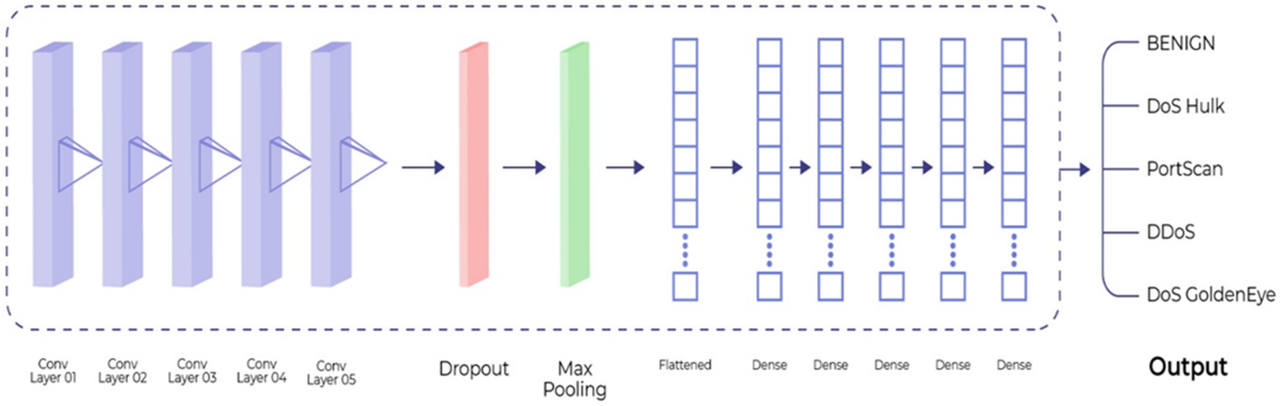
We developed a 1D-Convolutional Neural Network (1D-CNN) to identify local structural motifs within molecular fingerprints. This was the simplest deep-learning simplest model.The input bit vectors (1024-bit ECFPs) were transformed from 2D arrays into a 3D tensor format (1024) to facilitate feature extraction. The architecture employs 2 convolutional layers: a 64-filter layer followed by a 128-filter layer, both of which use a kernel size of 3 and ReLU activation. Each convolutional layer is accompanied with a MaxPooling1D layer (pool size 2) to reduce dimensionality and improve translation invariance, ultimately helping identify key motifs even if they appear at different bit positions. The extracted feature maps were flattened and processed through a 128-unit dense layer. Finally, a sigmoid-activated neuron performed binary classification. The model used the adam optimizer and Binary Cross-Entropy loss over a stratified split of training, validation, and test datasets (Fig. 4). Accuracy consistently layed around 50%, with higher precision (~60%) but very low recall (~10%).
2-D CNN
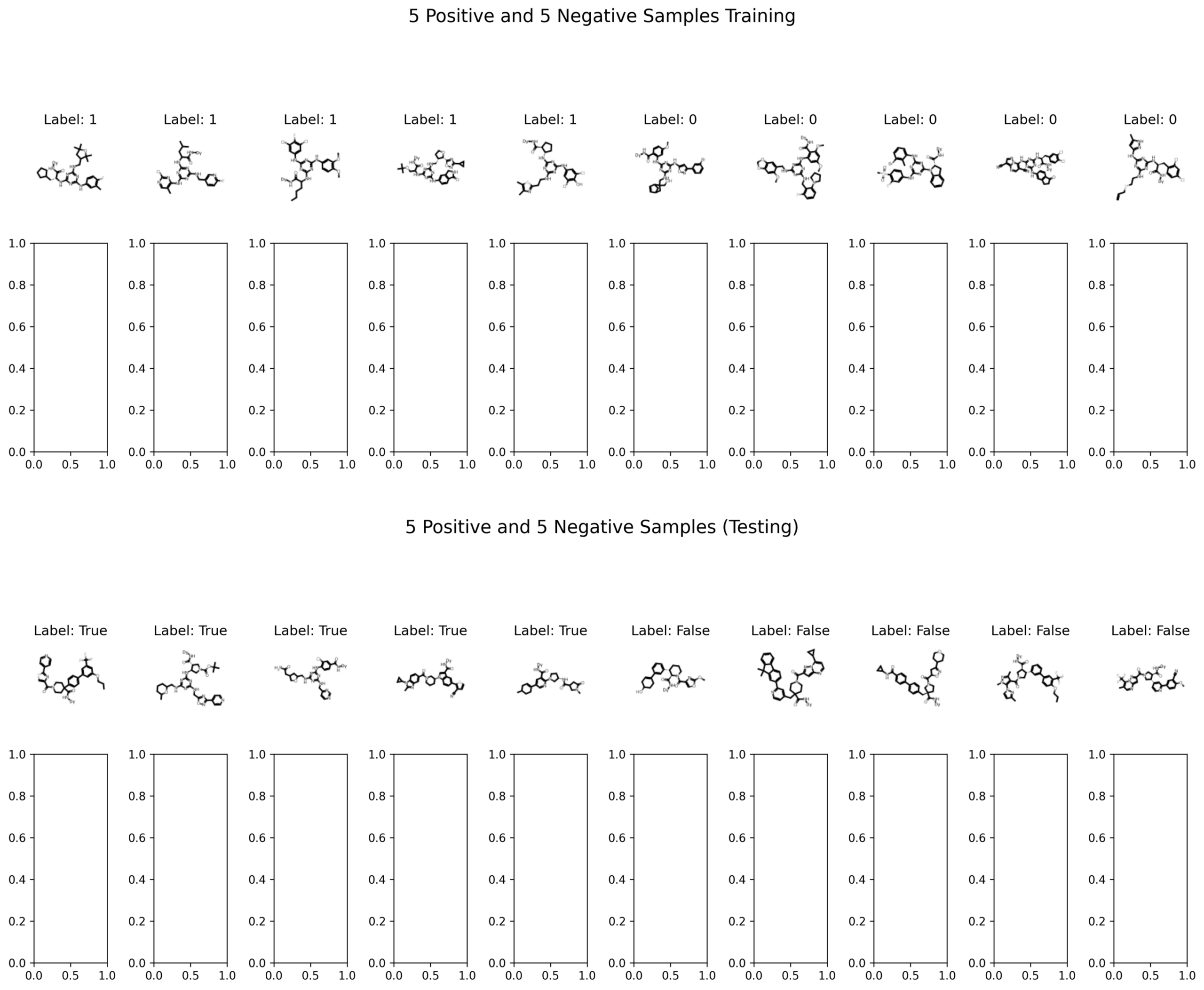
Rather than using ECFPs, the 2-D CNN uses generated image data via RDkit as input. The function MolToImage() converts molecules to images; then, the images must be preprocessed – they are resized to a target size, converted to grayscale, converted to a numpy array, and they have their pixel values normalized to the range [0,1]. 5 positive and 5 negative samples were selected from both training and testing datasets for display (Fig. 5).
The 2D CNN architecture analyzes this molecules represented as 100 x 100 x 1 grid-based images. It utilizes 3 convolutional layers involving 3×3 kernels (64, 64, and 128 filters) to extract spatial topological features. Moreover, we integrated batch normalization and 20% dropout layers to improve stability and generalization. To prevent overfitting, we introduced an ImageDataGenerator to perform real-time data augmentation. This generator performed rotations (20 degrees), horizontal flips, and spatial shifts to ensure orientation-invariance. Accuracy consistently layed around 55%, with higher precision (~60%) but very low recall (~20%). This result was expected, as although image-based molecular representations offer greater flexibility and potential to capture global visual patterns, they are often less chemically grounded than ECFPs (don’t preserve local chemical environments as well), leading to reduced robustness especially with limited training data.
Graph Neural Network
GNN models tend to perform better on molecular data because the structure of molecules is better represented through graphs rather than grids (i.e. images). The library used to construct this model was PyTorch Geometric, which is designed for deep learning on graphs. To convert the smiles data into graph representation, the function rdmolops.GetAdjacencyMatrix(mol) extracts bond connectivity to create edge indexes. In addition to extracting atomic numbers via atom.GetAtomicNum(), we expanded the node feature matrix by extracting local chemical properties including degree, hybridization, and aromaticity to reflect both chemical identity and connectivity of atoms. In the end, the function returns a PYG data object with x as the node and edge_index as the edge (Fig 6).
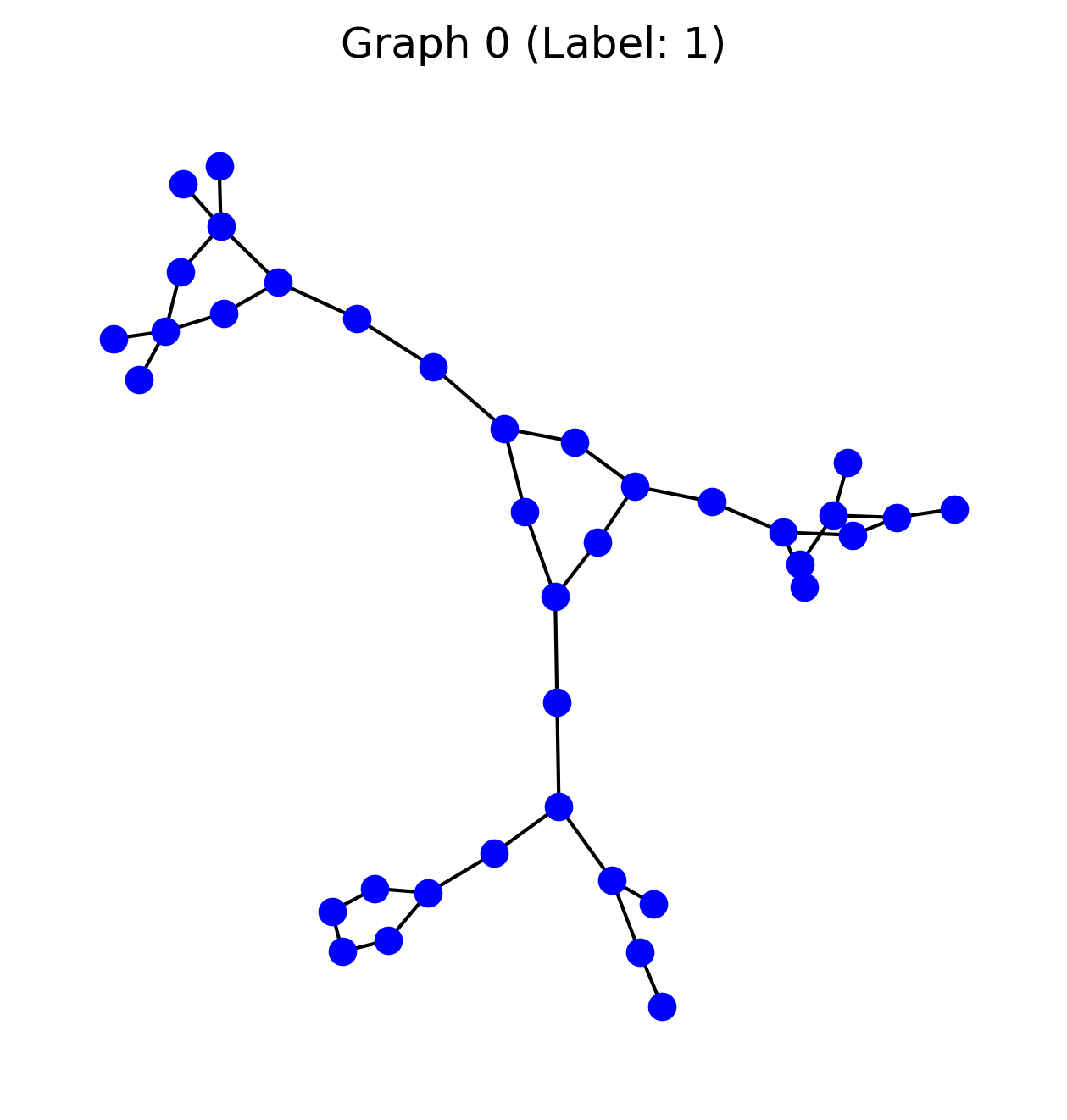
The GNN architecture consists of 3 sequential GraphConv layers (64, 128, and 64 hidden units). Graph Conv performs message-passsing updates by aggregating features from neighboring atoms along molecular bonds, enabling the model to capture local chemical environments. It does this by transforming atomic (node) features, updating the atomic (node) embeddings based on the surrounding chemical environment15, with ReLU acitivations applied after each layer. To generate a fixed-sized molecular embedding, we applied a global_max_pool layer followed by a 30% dropout for regularization. The model was trained using a binary cross-entropy loss function with the Adam optimizer over stratified datasets.
Ultimately, the GNN does very well at capturing local molecular structures. The forward pass of the model applies these 3 layers to the graph data. Global max pooling ensures the model aggregates the max feature of each node, creating a graph-level representation of the molecule.
Transformer Model
The Transformer architecture is built using TensorFlow and Keras to process ECFPs and metadata. Since ECFPs are fixed-length, non-sequential bit representations, we employ the self-attention mechanism not for its positional encoding mechanisms, but for its ability to globally aggregate information from the entire vector. In other words, the Transformer architecture doesn’t treat the fingerprint as a sequence, but rather as a collection of features. Thus, we apply Positional Encoding not to imply that there is a chemically-significant order, but rather to provide consistent index-level distinguishability across fingerprint dimensions, which are order–invariant. This allows the self-attention mechanism to learn relative importance of bits and co-occurrence patterns (i.e. bit position 80 and bit position 800 both “on” suggests global feature interaction).
First, the model defines the key hyperparameters: input_dim = 1024 (size of ecfp vector), D_model = 128 (transformer model size), num_heads = 2 (number of attention heads), DFF = 256 (size of feed-forward network), and num_layers = 4 (number of transformer layers). The Adam optimizer was utilized with a custom learning rate schedule, and the model was run for 12 epochs.
The TransformerEncoderLayer consists of a self-attention mechanism, multi-head attention mechanism, feed-forward network, layer normalization to stabilize training, and dropout. The self-attention aspect of transformers allows it to consider all substructures or chemical features (represented by bits) of a molecule simultaneously to get a better sense of chemical context, which other models often cannot do because they process data sequentially. This results in the capture of long-range dependencies, or relationships between distant features whose bits may be located far apart in the fixed-length vector of an input molecule. In the multi-head attention mechanism, each head looks for a specific chemical property or structural pattern. Inside each head there is a query, which describes what the model should pay attention to, keys to identify elements to pay attention to, values to average over, and finally a score function to apply the attention. By extracting separate aspects of input features, the transformer model captures richer interpretations of the ligand molecule. Ultimately, this mechanism also endows the model with interprepretability to provide new insights for drug discovery18.
The creation of the model itself involves multiple steps. The first step processes the ECFPs with transformer encoders, batch normalization and dropout, and dense layers. Global Average Pooling 1D is applied to reduce dimensionality. The second step is processing the metadata via dense layers and dropout. Initially, the function, calculate_descripters, returns the molecular weight, logP (hydrophobicity), and tpsa (topological polar surface area) of the molecule_smiles data to generate metadata descriptors aligned with the ECFP data. Finally, the ECFP and metadata representations are concatenated, and a final dense layer is applied to get the final binary classification output.
Hybrid GNN-Transformer Model
Like the name suggests, the GNNTransformer model is a novel hybrid approach that combines the best qualities of both the GNN and Transformer to maximize predictive ability. Just like the transformer itself, this model consists of multi-head attention applied into transformer encoder layers. However, rather than global average pooling, which merely computes the average over input features, we utilized attention pooling. Attention pooling assigns weights of importance to each feature and aggregates them, which ensures that the most crucial features dominate prediction. We clarify that the Transformer component is not intended to model sequential dependencies, as molecular fingerprints and physiochemical descriptors are fundamentally order-invariant. Rather, attention treats the input as a set to model higher-order dependencies between feature dimensions, with positional encoding functioning to provide index-level distinguishability.
To fuse the GNN and Transformer components into the hybrid model, we performed feature concatenation. Rather than feeding the GNN output into the Transformer, it processes 3 input streams in parallel. First, graph data passes through the GNN, resulting in a gnn_output vector. Separately, the ECFP fingerprints (ecfp_data) are projected into an embedding space and treated as feature tokens, each corresponding to a substructure bit-position. These embeddings are passed through the Transformer Encoder, condensed through Attention Pooling, and passed through the fully connected layer. Finally physical descriptors (metadata) are passed through a small MLP. Then, the extracted features are fused together, gluing them into a single feature vector. This final, fused vector is passed through a final linear layer, whose responsibility is to distribute weights to determine the relative importance of feature extractions (Fig. 7).
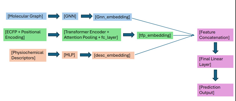
This model combines a diverse array of input representations. The GNN component incorporates graph representation for structural information. The Transformer component utilizes both molecular fingerprints and metadata descriptors, capturing relational codependence/co-occurence patterns and dependencies as well as physicochemical characteristics. Because it deals with a diverse range of inputs, the model had to make sure they were all the same length before combining them into single datasets.
Results
The majority of the models we explored displayed sup-par results with accuracy, precision, and AUC hovering at around 50%. Recall was often either frighteningly low at around 10%, suggesting that the models were over conservative (didn’t predict many positive outcomes), or extremely high, suggesting that the models were overfitting.
The GNN Transformer model performed the best by far. Every single metric improved significantly from the baseline on all 3 proteins, demonstrating its strong predictive power and potential generalization capability on protein-ligand binding classification. As displayed by the confusion matrices, accuracy, precision, recall, AUC, and F1_score improved by 20-30%. Average precision improved by approximately 20% (Fig. 8-10). Since we applied scaffold-based partitioning to the training and testing datasets instead of random sampling, we witnessed a slight reduction in overall performance compared to random sampling, showing that previously our model was essentially memorizing scaffold patterns, leading to inflated performance. While accuracy and precision decreased, AUC and Average Precision remained high or increased, indicating that the model successfully ranks binders above non-binders for novel scaffolds. Accuracy and precision are threshold dependent, meaning they depend on a probability cutoff and can be misleading in imbalance datasets. Thus, AUC and Average Precision, which rank performance in the context of class imbalance and across threshold, are generally more important for drug discovery.
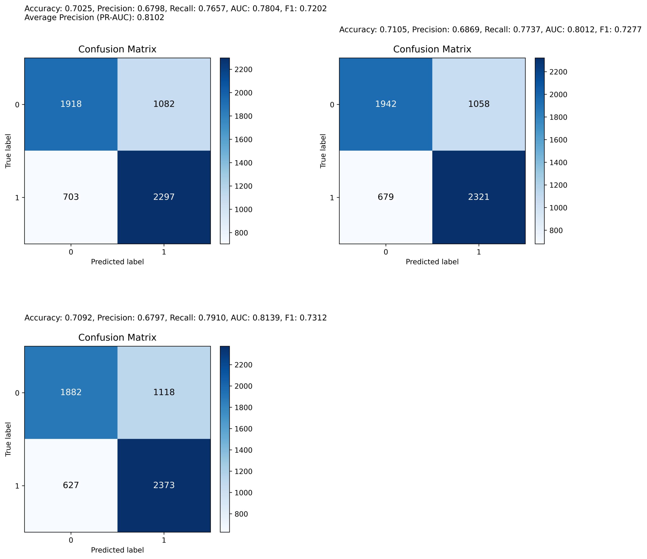
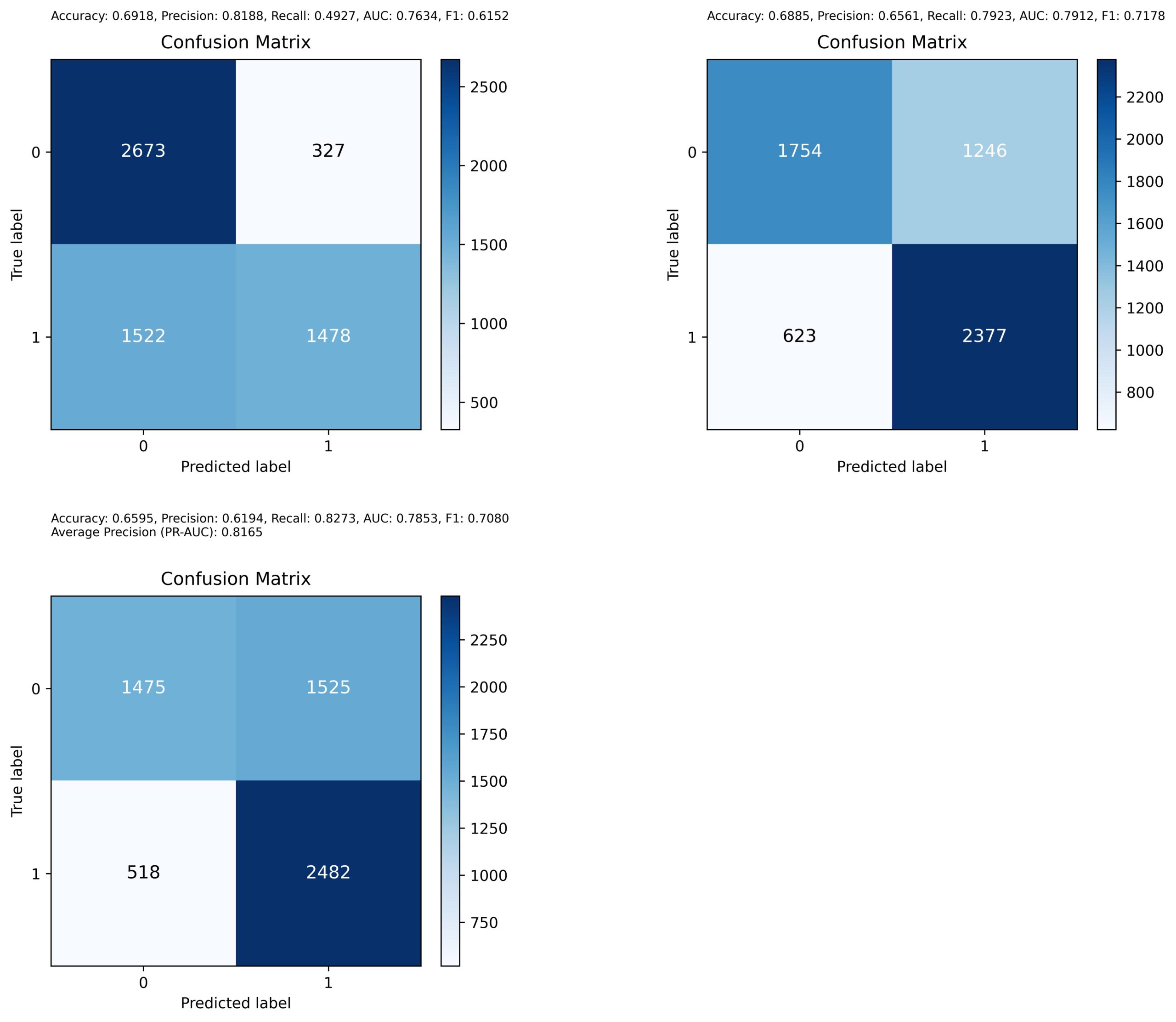
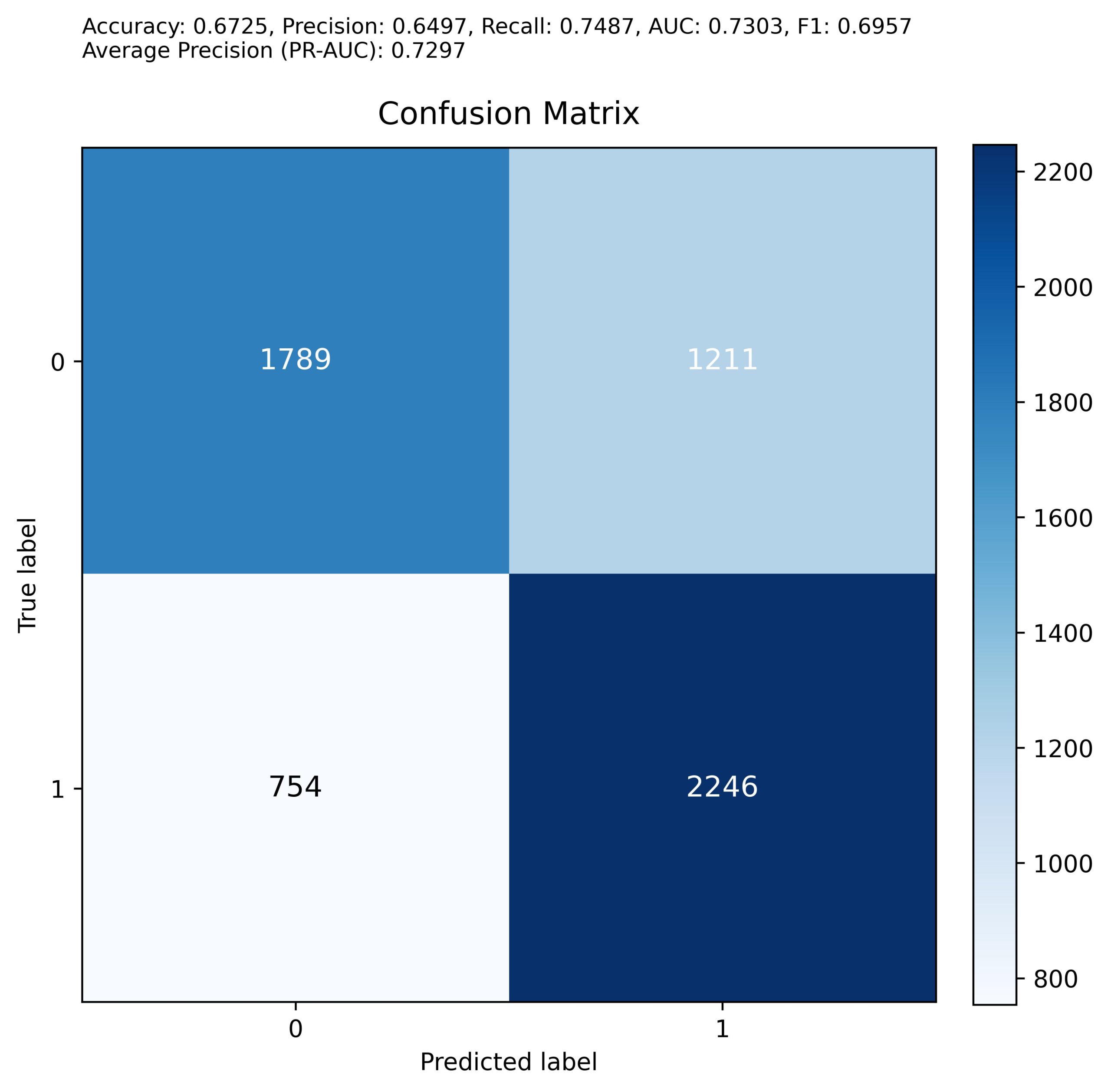
Summary of Results (Approximate Averages)
The following table displays the approximate average values of each metric for the 3 target proteins:
| | Accuracy | Precision | Recall | AUC | F1_score | Average Precision |
| HSA | 0.71 | 0.68 | 0.78 | 0.80 | 0.73 | 0.81 |
| BRD4 | 0.68 | 0.77 | 0.68 | 0.78 | 0.68 | 0.82 |
| sEH | 0.67 | 0.65 | 0.75 | 0.73 | 0.69 | 0.73 |
Comparison with state-of-the-art pipelines
Having established a satisfactory baseline performance, we then evaluated the performance of our GNN transformer compared to previous binary classification pipelines. For this, we selected two deep learning models for comparisons: the NeurlIPS 2024 Belka competition 11th place solution and a 1D-CNN Transformer, both of which were trained and tested on the same dataset (BELKA) with the same protein targets. All comparisons were conducted under matching conditions. Models were evaluated on the same dataset, target labels, and evaluation metrics defined by the Kaggle competition. However, these competing solutions should be treated as a contextual benchmark rather than a direct architectural comparison, as they were developed under the same competition constaints but with different modeling choices.
| Method | Average Precision |
| 1D-CNN Transformer | 0.64 |
| Belka 11th Place Solution | BRD4: 0.64 HSA: 0.39 seH: 0.93 |
The 1D-CNN Transformer approach, done by Mert Byrjtrm, focused on encoding SMILES strings and incorporating physicochemical features into the building blocks19. The model achieved an AP score across all 3 target proteins of 0.64, which is lower than our achieved AP scores of 0.81 for HSA, 0.82 for BRD4 and 0.73 for sEH (Table 2).
The NeurlIPS 11th Place solution employed Embedding + MLP models on building block IDs (3 building blocks construct a molecule)20. The results for Average Precision are severely asymmetrical, as illustrated by the clearly disproportionate results for different proteins. Although the AP for seH is higher than the results we received, our model still outperforms since it demonstrates stronger consistency on all 3 proteins, which makes it significantly more reliable in the drug-discovery pipeline. Also, our AP values of around 0.7 are higher than both the AP values of BRD4 and HSA of 0.64 and 0.39 respectively (Table 2).
Results Discussions
The GNNTransformer outperformed baseline models mainly because it incorporates a variety of complementary input representations. Graph representation, molecular fingerprints, and metadata descriptors combine to capture all aspects of the molecule being analyzed. Graph data captures structural information of a molecule, especially connectivity between atoms, which helps the model understand local relationships. ECFPs capture specific sequential patterns; then, the transformer does a great job at capturing long-range interactions/dependencies. Metadata descriptors provide physicochemical properties which the other 2 representations lack. Finally, the GNNTransformer finds relationships between all 3 features to predict binding affinity.
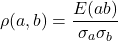
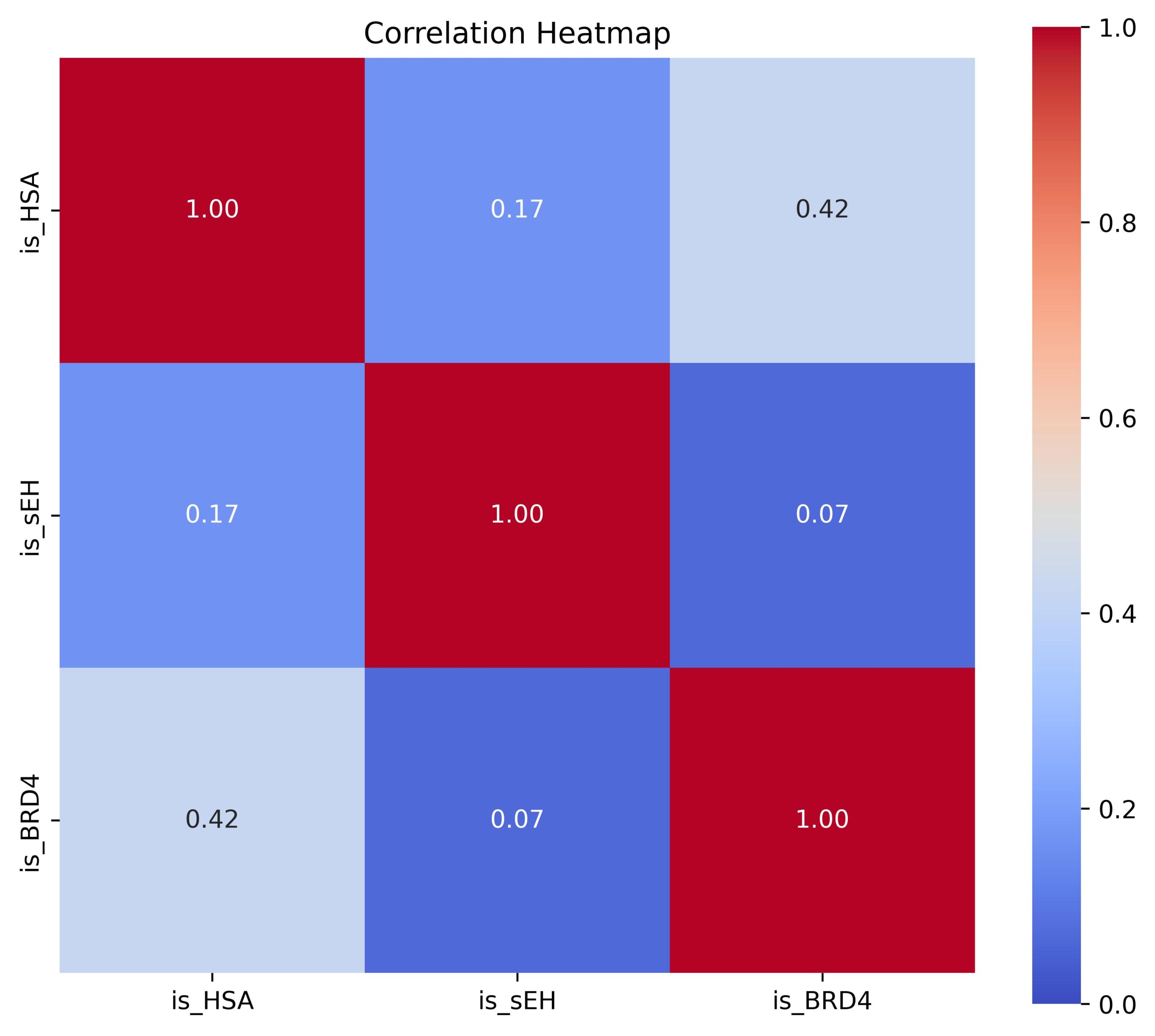
Overall, our model achieved ~70% precision, recall, F1_Score, and accuracy, 80% AUC, and 70-80% AP for all three proteins, which is a significant improvement over baseline models and outperforms several competing methods (Table 1). However, many limitations still persist. For one, our model is trained on binding data for only a few target proteins, limiting generalizability to still unknown protein families. Even so, our model exudes convincing potential that it has the ability to perform on a similar level across a wide-range of diverse types of proteins. This predictive potential can be illustrated using the protein correlation heat-map (Fig. 11), which shows the degree of similarity of the proteins in terms of their binding behavior across a set of ligands. Each entry is the Pearson correlation coefficient between protein a and protein b21.
(1) 

HSA and BRD4 have relatively similar binding profiles — they bind to similar molecules — with a correlation coefficient of 0.42. This may reflect underlying biological similarities between the 2 proteins — BRD4 binds to acetylated histones in transcriptional regulation, while HSA transports hydrophobic molecules in the bloodstream. As such, both bind to small, hydrophobic/aromatic ligands7. In contrast, sEH behaves quite differently from HSA and BRD4 with a correlation coefficient of 0.07 compared to BRD4 and 0.17 compared to HSA. This may reflect the fact that seH is an enzyme that binds to more polar molecules such as epoxides and requires structurally specific substrates7.
The fact that the GNN Transformer demonstrated similar improvements on seH in comparison to HSA and BRD4 despite their striking structural and functional differences suggests that our model has the potential to perform well on out-of-distribution proteins. However, this must be tested on a separate dataset.
Conclusion
For protein-ligand binding affinity prediction, the GNNTransformer algorithm uses multi-modal molecular features and physicochemical characteristics. This model distinguished itself from previous models in three major aspects. First, it integrated multi-dimensional, complimentary, input representations: namely graph data, metadata, and ECFPs. This allowed for the extraction of information of different scales and the identification of relationships between features. Secondly, it extracted physicochemical characteristics beyond the SMILES data and raw structure, providing additional chemical context. Thirdly, the transformer component’s multi-head attention mechanism extracted different aspects of the most important features simultaneously, which assisted the learning of complex patterns (long-range dependencies) and generalization. Finally, we tackled class imbalance via batch balancing and threshold tuning.
Under a scaffold-based split, threshold-dependent metrics (accuracy, precision) decreased due to distribution shift, while ranking-based metrics (ROC-AUC, Average Precision) remained stable or improved, indicating preserved enrichment and generalization to novel chemical scaffolds.
Key takeaway: By optimizing feature selection, learning complex patterns and relationships, and addressing class imbalance, the GNN Transformer achieved a 20-30% improvement over baseline across a wide range of metrics, particularly AUC and Average Precision, and across three structurally diverse proteins, demonstrating greater reliability in identifying potential drug candidates.
Future Work
Although the present architecture predicts similarly well on HSA, BRD4, and sEH, which have been established to be structurally heterogeneous, it is still possible that the model does not perform as well on different proteins. As such, the logical next step would be to test our GNN Transformer on proteins from external datasets to confirm that the model is indeed capable of performance on a large-scale. The model may also benefit from the incorporation of protein sequence and/or structural data. Currently, the present architecture relies solely on ligand sequence, structural, and physicochemical data to predict binding affinity between the ligand and its protein. This method is simpler, but it assumes that binding is mainly determined by ligand structure and may miss important protein-ligand interactions. By integrating protein features, performance of the model may increase, improving generalization across different protein variants.
It may be essential to focus on crucial residues of the protein pocket22. which directly interact with the ligand through hydrogen bonds, van der Waals forces, and hydrophobic interactions. These protein pockets generally have different geometric and chemical characteristics compared with non-pocket regions. Thus, effectively representing the features of protein pockets is a critical next step23.
It’s imperative to acknowledge that our model is not sensitive to mutations in the protein, involving single or several amino acid changes. Thus, it would be crucial to screen for and detect observable changes in affinity when mutations occur. There also exists the problem of “undruggable” proteins, a class of proteins often characterized by large, complex structures and functions, which are difficult to tackle using conventional targeting strategies24.
Moreover, our model solely looked at non-covalent interactions; however, there could be potential cases of covalent binding, which has gained increasing attention in the field of drug development. Novel competing models like TEFDTA, which incorporates fingerprint transformation and Transformer encoder modules, takes advantage of covalent binding data to enhance predictive ability25.
Instead of tackling the binding prediction issue using classification, we may transition to regression modeling, utilizing the dissociation constant values (Kd) of already-known protein-ligand pairs for a more realistic and nuanced approach.
Finally, our models are static – they don’t capture dynamic molecular interactions. This problem could potentially be solved through equivariant GNN’s, which capture 3D molecular interactions, and reinforcement learning, which rewards or punishes models based on their actions (i.e. changing the orientation of a bond)26.
Acknowledgements
I would like to thank Inspirit AI for providing me with resources and my mentor Sriram Hathwar for all his guidance and support through the research process.
References
- Kaur, Navjeet, et al. “Small molecules as cancer targeting ligands: Shifting the paradigm.” Science Direct, vol. 355, 2023 [↩]
- Zhao, Lingling, et al. “A brief review of protein–ligand interaction prediction.” Science Direct, vol. 20, 2022. [↩]
- Li, Shuya. “MONN: a multi-objective nueral network for predicting compound-protein interactions and affinities.” Cell Systems, vol. 10, no. 4, 2020 [↩]
- Wang, Kaili, et al. “DeepDTAF: a deep learning method to predict protein–ligand binding affinity.” Briefings in Bioinformatics, vol. 22, no. 5, 2021 [↩] [↩] [↩]
- Velazquez-Campoy, Adrian, and Ernesto Freire. “Isothermal titration calorimetry to determine association constants for high-affinity ligands.” Nature, 2006 [↩]
- Maynard, Jennifer A., et al. “Surface plasmon resonance for high-throughput ligand screening of membrane-bound proteins.” Biotechnology Journal, vol. 4, no. 11, 2009 [↩]
- Blevins, Andrew. “NeurlIPS 2024 – Predict New Medicines with BELKA.” Kaggle, 2024 [↩] [↩] [↩]
- Weininger, David. “SMILES, a chemical language and information system. 1. Introduction to methodology and encoding rules.” ACS Publications, vol. 28, no. 1, 1988 [↩]
- Wu, Hongjie, et al. “AttentionMGT-DTA: A multi-modal drug-target affinity prediction using graph transformer and attention mechanism.” Science Direct, vol. 169, 2024 [↩]
- Wang, Huiwen. “Prediction of protein–ligand binding affinity via deep learning models.” Briefings in Bioinformatics, vol. 25, no. 2, 2024 [↩] [↩] [↩]
- Arcon, Juan Pablo, et al. “Molecular Dynamics in Mixed Solvents Reveals Protein–Ligand Interactions, Improves Docking, and Allows Accurate Binding Free Energy Predictions.” ACS, vol. 57, no. 4, 2017. [↩]
- Dandibhotla, Somanath, et al. “GNNSeq: A Sequence-Based Graph Nueral Network for Predicting Protein-Ligand Binding Affinity.” Pharmaceuticals, vol. 18, no. 3, 2025 [↩]
- Wang, Guishen, et al. “DeepTGIN: a novel hybrid multimodal approach using transformers and graph isomorphism networks for protein-ligand binding affinity prediction – Journal of Cheminformatics.” Journal of Cheminformatics, 29 December 2024 [↩] [↩]
- Lv, Zhibin, et al. “Anticancer peptides prediction with deep representation learning features.” Bioinformatics, vol. 22, no. 5, 2021 [↩]
- Wang, Yuxiao, et al. “Prediction of protein-ligand binding affinity with deep learning.” ScienceDirect [↩]
- Hahn, Mathew. “Extended-connectivity fingerprints.” PubMed, 24 May 2010 [↩]
- Qazi, Emad, et al. “A One-Dimensional Convolutional Neural Network (1D-CNN) Based Deep Learning System for Network Intrusion Detection.” MDPI, 2022. [↩]
- Hu, Haohuai, et al. “NHGNN-DTA: a node-adaptive hybrid graph neural network for interpretable drug–target binding affinity prediction.” Bioinformatics, vol. 39, no. 6, 2023 [↩]
- “NeurIPS-2024—Predict-New-Medicines-with-BELKA-COMPETITION.” Github [↩]
- Hồng, Đăng Nguyễn. “11th place solution – SSL Pretraining, Multi-models, Multi-representations and Luck.” NeurIPS 2024 – Predict New Medicines with BELKA [↩]
- Benestey, Jacob, et al. “Pearson Correlation Coefficient.” Springer Nature, 2009 [↩]
- Mareuil, Fabien, et al. “Protein interaction explorer (PIE): a comprehensive platform for navigating protein–protein interactions and ligand binding pockets.” Bioinformatics, vol. 40, no. 7, 2024 [↩]
- Li, Shuya, et al. “PocketAnchor: Learning structure-based pocket representations for protein-ligand interaction prediction.” Cell Systems, vol. 14, no. 8, 2023 [↩]
- Xie, Xin, et al. “Recent advances in targeting the “undruggable” proteins: from drug discovery to clinical trials.” Nature, 2023 [↩]
- Li, Zongquan, et al. “TEFDTA: a transformer encoder and fingerprint representation combined prediction method for bonded and non-bonded drug–target affinities.” Bioinformatics, vol. 40, no. 1, 2024 [↩]
- Chen, Shihong, et al. “Local–Global Structure-Aware Geometric Equivariant Graph Representation Learning for Predicting Protein–Ligand Binding Affinity.” IEEE Transactions on Neural Networks and Learning Systems, vol. 36, no. 8, 2025 [↩]