Allocating Public Resources for Maximum Societal Benefit: An Optimization Approach to County Budgeting

Abstract

This study develops and applies an award-function optimization model to the allocation of budget surplus across five public service domains in Fairfax County, Virginia. This is particularly timely given that Fairfax County adopted its FY 2027 Budget on May 5, 2026. Drawing on a qualitative synthesis of peer-reviewed evidence from education economics, public health, public safety, social services, and economic development, the model parameterizes budget sensitivity weights (α) and diminishing returns factors (β) for each domain. These weights are author-assigned and evidence-informed rather than econometric estimates. This study presents an optimization model to maximize a concave award function, subject to a fixed surplus constraint, which is solved numerically via a bisection algorithm and tested under four alternative weighting scenarios (baseline, equal α, health-first, and equity-first) and Monte Carlo parameter perturbation reflecting Fairfax’s policy priorities. Analysis revealed that all optimized allocation strategies match or outperform their own equal-dollar baseline, with gains ranging from 0.000 to 0.064 on the societal benefit index (a dimensionless 0–1 model score in which higher values indicate greater modeled benefit). Specifically, the literature-derived baseline scenario yielded a gain of 0.056 (0.402 vs. 0.346 under uniform allocation). Furthermore, two illustrative allocations are proposed: the baseline, where 60.9% of the surplus goes to schools, and the health-first, which attains the highest model score among the scenarios tested (0.418). Overall, this framework offers a tool that other local governments can replicate for evidence-based budgeting.

Keywords: budget optimization, award function, public investment, diminishing returns, evidence-based policy, municipal finance, resource allocation.

Introduction

Governments around the world are continually confronted with the problem of deciding what to do with a limited public budget in the face of competing demands for it, with the ultimate goal being to maximize the overall contribution of the public budget to society’s welfare. The challenge has been further compounded in the last thirty years, as financial pressures have increased and the needs of public services have grown^1,2. The Organization for Economic Co-operation and Development (OECD) has pointed out that government spending is an important driver of societal returns, and the empirical growth literature separates out productive expenditures (e.g., infrastructure, human capital, health) from less productive administrative or redistributive expenditures^3,4,5. Economic literature has already shown that the law of diminishing returns is a general law in economics and is relevant for public expenditures as well: for every additional dollar of spending in a given area, the marginal gain is likely to diminish with every dollar of spending^4,6. This relationship, which is most often modeled as a concave production function, has materialized across multiple domains of government activity, including education^7,8, public health^9,10, and safety^11,12. Therefore, it is unlikely that a uniform allocation of budget, in which all domains receive equivalent amounts of money, is optimal, due to the fact that it largely fails to account for heterogeneous returns across spending categories. In the United States specifically, local governments are responsible for a disproportionate share of direct public service delivery, including K-12 education, policing, public health, and social services¹³. Despite this, budget allocation at the county level is often driven by incremental adjustments to prior-year spending, known as “incremental budgeting,” rather than a systematic analysis of where marginal dollars produce the greatest benefit^14,15.

Problem Statement

Fairfax County, Virginia, presents an interesting case study for evidence-based budget optimization. With over 1.15 million residents, a median household income of $154,545, and a rate of 66.3% of adults possessing a bachelor’s degree or higher¹⁶, the county’s General Fund Budget is approximately $5.96 billion for FY 2027¹⁷. In particular, the county allocates a total of $4.34 billion annually across the five domains analyzed in this study, consisting of public safety, health, social services, K-12 education, and economic development¹⁷. However, the county faces several fiscal pressures that are compounding. Based on recommendations from the Joint Legislative Audit and Review Commission’s review of Virginia’s K-12 funding in education, Fairfax County Public Schools estimates that the division faces a chronic underfunding gap of $568.7 million per year relative to what JLARC’s proposed funding standards would provide^18,19. At the same time, the county is home to nearly 80,000 federal employees who are facing potential workforce reductions²⁰, and demand for emergency housing and social services has been characterized as “sustained” and “unprecedented” by the county’s own budget documents¹⁷. In the FY 2027 Advertised Budget, the County Executive identified that there was a balance of $23.17 million remaining for theBoard of Supervisors’ consideration, representing approximately 0.39% of the $5.96 billion General Fund and a discretionary surplus that the Board had to allocate across the numerous competing priorities¹⁷. However, the issue lies in how to optimally distribute this surplus to maximize the societal benefit index.

Research Objectives

There are three primary objectives to this study. The first is to develop a mathematical optimization framework that incorporates domain-specific sensitivity weights and diminishing return parameters that are informed by peer-reviewed literature. The second is to apply this framework to Fairfax County’s FY 2027 budget surplus, and identify the optimal allocation of $23.17 million across the five public service domains. The third is to compare the performance of four alternative scenarios, with each optimized scenario evaluated against its own
equal-dollar (uniform) baseline, ultimately evaluating the robustness of the optimization approach across different policy priorities.

The five domains were chosen because they encompass major discretionary spending categories in the county’s General Fund for which there is peer-reviewed evidence on the returns to marginal spending in measurable welfare outcomes, in contrast to the fixed-cost categories like debt service, employee benefits, and judicial administration, which do not lend themselves to marginal benefit analysis (see the Scope and Delimitations). The four alternative scenarios were selected to cover the policy space the Board of Supervisors might plausibly explore: a non-optimized uniform allocation, an equal-α scenario to control for the effect of only β heterogeneity, and two alternative priority weighted scenarios (one health-first and one equity-first) which show two competing normative framings often discussed in local budget debates.

Research Questions

The study addresses two research questions. First, does an evidence-based, optimized allocation of budget surplus generate a higher societal benefit index value than uniform distribution across the service domains? Second, how do alternative weighting scenarios depending on varying policy priorities compare on the societal benefit index, and which produces the maximum benefit?

Significance of Study

This research will contribute to existing literature by providing a mathematically grounded framework that local governments can adopt without econometric expertise. While previous optimization literature in operations research has addressed resource allocation under concavity constraints²¹, applications to municipal budget allocation using evidence-informed parameters remain sparse. Thus, this paper aims to bridge the gap between previous academic research on public spending elasticities and budget decision-making at the local government level. The findings will be especially notable and relevant to the Fairfax County Board of Supervisors, who deliberated the allocation of the FY 2027 budget surplus. More broadly, the framework will also be generalizable to any jurisdiction where domain-specific spending elasticities can be estimated in accordance with previous literature.

Scope and Delimitations

This study explores the allocation of discretionary budget across five service domains made up of public safety, health, social services, K-12 education (FCPS), and economic development. The analysis does not cover the full General Fund, excluding categories such as judicial administration, legislative functions, debt services, employee benefits, and more, which are either fixed costs or do not lend themselves to marginal benefit analysis. The model uses a formula that allocates surplus in accordance with the respective domain’s share of the total surplus, rather than its share of the existing budget, in order to avoid systematically penalizing large departments. This design choice is further discussed in the Methods. Finally, parameter values are determined from pre-existing literature rather than original econometric estimation.

Returns on Education Spending

In public economics, there has been vast research regarding the relationship between school spending and school outcomes. The Coleman Report has been the source of skepticism about the effectiveness of public investments for several decades, as it suggested that the resources schools provide did not seem to contribute to student achievement in ways that were independent of family background and social context²². This skepticism continued with Hanushek, who observed that a systematic relationship between school resources and student performance does not exist²³ and that “simply providing more funding or a different distribution of funding is unlikely to improve student achievement”²⁴. This was a common theme during the early 2000s debates on education policy, and remains true to this day for arguments calling for education spending restraints²⁵. Despite this, more recent studies have greatly challenged this conclusion. Jackson, Johnson, and Persico exploited the timing of court-mandated school finance reforms across U.S. states to estimate the causal effect of spending on long-term outcomes²⁶. They discovered that a 10% increase in per-pupil spending over a 12-year time period corresponded with 0.31 additional years of completed education, approximately 7% higher adult wages, and a 3.2 percentage-point reduction in the incidence of adult poverty²⁶. These effects were prominent in lower-income families. Jackson and Mackevicius conducted a comprehensive meta-analysis of school spending evaluations in the United States, which confirmed that the causal effects of school spending on educational outcomes are positive⁷. Lafortune, Rothstein, and Schanzenbach corroborated these findings by using post-1990 school finance reforms, documenting that reform-induced spending increases improved student achievement in terms of standardized test scores⁸. At the state level, the Joint Legislative Audit and Review Commission identified that Virginia’s K-12 school divisions are chronically underfunded, with several Great Recession-era changes alone reducing state funding by $487 million statewide¹⁸, which is the source of the county’s $568.7 million annual funding gap noted above¹⁹. This finding is also consistent with broader evidence stating that spending cuts in education generate measurable harm to student outcomes²⁷, harms that extend to education’s broader civic and democratic processes²⁸, particularly in high-cost jurisdictions where teacher labor markets are competitive, such as FCPS. However, while it is clear that additional budget allocation in education would be beneficial, it remains nuanced with respect to diminishing returns in education. The returns to investments in school spending are not identical: Baron found that the benefit from an increase in the amount of operational spending was large for test scores, dropout rates, and postsecondary enrollment, whereas an increase in capital expenditures was relatively small, suggesting that the marginal benefit of a dollar of education spending varies with the nature of spending²⁹. However, Jackson et al. found sustained returns even at relatively high baseline spending levels, which complicates that picture and suggests that the point of sharply diminishing returns has not been reached in most U.S. school districts²⁶. Rothstein and Schanzenbach further confirmed that school finance reforms after 1990 produced significant attainment and earning effects, which reinforces the idea that educational spending remains productive at current levels³⁰. Several studies have documented that increased spending in less affluent areas can enhance equality, and targeted spending in disadvantaged communities can yield disproportionately high returns^8,26,31,32. Collectively, the strength and consistency of the evidence related to returns in educational spending, combined with the severity of the FCPS underfunding gap, inform the assignment of the highest α (0.33) and near-linear β (0.75) to the education domain in the model. These studies estimate elasticities for general school spending rather than marginal surplus allocation specifically; the mapping from published elasticity estimates to the model’s β parameter is therefore qualitative rather than formally derived, a limitation later discussed.

Returns on Public Health Investment

Similar questions about marginal returns arise in public health, where returns to investment have been assessed through a variety of metrics, including mortality reduction, morbidity prevention, and healthcare cost avoidance. Masters, Anwar, Collins, Cookson, and Capewell conducted a systematic review of 52 studies examining the return on investment (ROI) of public health investment in high-income countries such as America⁹. They found a median overall ROI of 14.3:1, with local public health investments returning a ratio of 4.1:1 and national interventions returning 27.2:1. Mays and Smith examined the relationship between local public health spending and preventable mortality using a panel of U.S. communities over the period of 13 years¹⁰. Their findings suggest that each 10% increase in local health spending was associated with a 6.9% decline in infant mortality, a 3.2% decline in cardiovascular disease mortality, a 1.4% decline in diabetes mortality, and a 1.1% decline in cancer mortality. Another study found that counties in quartile 2 of investments in the social determinants of health (SDOH) had an average of 9.09 fewer overdose deaths per 100,000 population, along with 13.18 and 13.92 in quartile 3 and quartile 4 respectively³³. Similarly, Sowmyan et al. concluded that a one-standard-deviation increase in per-capita total expenditures was linked to a reduction of 0.51 deaths per 1,000 live births³⁴. Together, these studies indicate that public health spending has an independent protective association with public health. Singh conducted a complementary systematic review of public health spending and population health outcomes³⁵. In the review, they synthesized 17 empirical studies and 5 literature reviews, concluding that increases in public health spending are more generally correlated with greater population health. Leider, Alfonso, Resnick, and McCullough evaluated the value of 40 years’ worth of local public health spending and estimated that the benefits of the mortality savings from continuous local public health spending outpaced its costs³⁶. More recently, Turner et al. reviewed 118 ROI analyses of health interventions published between 2018 and 2021, finding wide methodological variation across studies, though the broader literature consistently reports positive returns for preventative health investments³⁷. Bekemeier, Grembowski, Yang, and Herting also demonstrated that specific local public health activities, such as maternal and child health services, are accompanied by reductions in racial disparities in mortality outcomes³⁸. Hence, the convergent evidence of positive, yet also moderately diminishing local returns, informs the assignment of α (0.22) and β (0.65) to the health domain in the model. It should be acknowledged that ROI estimates such as the 14.3:1 figure from Masters et al. are drawn primarily from intervention-specific studies (e.g., vaccination programs, smoking cessation) rather than general local public health department budgets; the mapping from these intervention-level returns to the model’s domain-wide β parameter therefore carries additional uncertainty, consistent with the broader limitation discussed in the Limitations.

Public Safety Spending

Turning from health to safety, the latest research on the effects of police resources on crime has produced increasingly credible causal estimates. Chalfin and McCrary analyzed police and crime data for 242 large U.S. cities from 1960 to 2010, and they estimated a cost-weighted crime elasticity with respect to police of approximately -0.5¹¹. This means that each time the police force size is increased by 10% the cost-weighted sum of crimes is reduced approximately by 5%. They also calculated that for each $1 of extra policing, the estimated value of the resulting social benefits is $1.63, most of which comes from fewer incidents of violent crime. Mello also used Community Oriented Policing Service data from the federal government, finding crime-police elasticities of approximately -1.3 for violent crime and -0.8 for property crime¹². This implies an estimated social return of $352,000 in reduced victimization costs per additional officer. The evidence indicates that the returns to police spending continue to be positive, but could have more pronounced diminishing returns than education or health spending. Chalfin and McCrary observed a negative relationship between marginal productivity of police and the number of police¹¹. Evans and Owens documented that COPS hiring grants increased police force size and reduced crime, while Lee, Eck, and Corsaro conducted a systematic review with findings that suggested mixed results depending on methodology, thus underscoring the difficulty of isolating causal effects in policing research^39,40. Piza and Chillar provided further evidence by studying mass police layoffs in New Jersey, concluding that reductions in police force size corresponded with sizable increases in crime⁴¹. Ultimately, these findings support the assignment of α (0.18) and the relatively lower β (0.55) to the public safety domain in the model, reflecting more sharply diminishing returns compared to education or health. It should be acknowledged that the cited elasticities pertain specifically to police labor rather than the full public safety budget category modeled here, which also encompasses fire and rescue, emergency management, and prevention-oriented programs that may exhibit different marginal returns; the mapping from police-labor elasticities to the broader domain β parameter therefore carries additional uncertainty, consistent with what is discussed in the Limitations.

Social Services Spending

Social services at the county level encompass child welfare, family support, housing assistance, and community development programs. A growing body of literature indicates that county-level social spending produces measurable improvements in welfare outcomes. A cross-sectional study of county-level government expenditures and healthcare utilization among low-income Medicare beneficiaries found that high spending on housing and community development was associated with 11% higher rates of primary care visits, and higher spending in community development and public transit also was associated with 6-10% lower preventable hospital rates⁴². This suggests that, by investing in local social services, a county can reduce long-term costs as a result of a decrease in hospitalizations and visits. Bradley et al. examined the ratio of social services spending to healthcare spending across the U.S. and found that states allocating a higher proportion to social services relative to healthcare had significantly better health outcomes, including lower adult obesity rates and lower mortality from causes such as lung cancer, acute myocardial infarction, and type 2 diabetes⁴³. Cardona et al. determined that, in urban counties, a one-standard-deviation increase in spending on building infrastructure was linked to an increase in Life Expectancy at Birth (LEB) by 1.14 years in 2005 and 1.05 years in 2010⁴⁴. Therefore, long-term social investments in housing, nutrition, and family support may be more cost effective at improving population health than the equivalent of increases in direct healthcare spending. In child welfare in particular, the NSCAW III Child Welfare Workforce Study examined child welfare worker burnout and found that 74.9% of supervisors identified job stress and burnout as the primary reason for caseworker turnover, with workload cited by 41.3% of respondents⁴⁵. This indicates that staffing capacity is also a limiting resource in child welfare service delivery and that workload-related turnover is likely to be a potential pathway through which increased investment in staffing could enhance service continuity for vulnerable populations. Research from Lee, Kirkland, Miranda-Julian, and Greene also highlights how mothers who received in-home services were half as likely to be confirmed subjects for physical abuse or neglect by their children’s seventh birthday compared to the control group⁴⁶. Fowler and Chavira found that housing services decreased the risk of child welfare families being placed in foster care and homelessness, showing that investing in supportive social services infrastructure can not only lower the risk of children leaving care into more expensive downstream services, but can also prevent the service altogether⁴⁷. Theories imply a moderately concave relationship, which is not as well supported empirically as are the theories regarding the education-health returns. The evidence on workload-driven turnover and on the effects of incremental home-visitation and housing services^45,46is consistent with the expected concavity in the return of these services as caseloads increase to families with less severe needs, based on these studies’ findings of roughly proportional returns over a range of caseloads, although the concavity is an interpretive judgment, not a direct finding of these studies. Hence, we assign the associated variables α and β to 0.22 and 0.70 respectively to the social services domain of the model, reflecting moderate priority and moderately sustained returns.

Economic Development Spending 

The final domain, economic development, typically comprises business attraction incentives, workforce development programs, and infrastructure investments aimed at expanding the tax base. The literature on the effectiveness of local economic development incentives is much more skeptical compared to literature on education, health, social services, or public safety spending. Bartik conducted a comprehensive review of place-based economic development policies and concluded that while targeted incentives can produce positive employment effects, the returns diminish rapidly as programs scale, with many incentives just serving as transfers to firms that would have invested anyway⁴⁸. Kenyon, Langley, and Paquin similarly found that tax incentive programs for economic development often fail cost-benefit tests, particularly when opportunity costs are considered⁴⁹. At the county level, the FY 2027 Advertised Budget Plan characterized the impact of proposed budget reductions in economic development programs as “limited,” suggesting that the county’s own assessment reflects the fact that there are low marginal returns from incremental spending changes in this domain¹⁷. This is consistent with broader literature findings that wealthy, high-amenity jurisdictions like Fairfax County already have strong locational advantages, and therefore there is less marginal value in additional economic development spending^50,51. These findings support the idea that the economic development domain will have the lowest sensitivity weight (α) of 0.05, and the most sharply diminishing β (0.45) in the model.

Diminishing Returns in Public Expenditure

Across all five domains, the principle of diminishing returns in government spending is well established within the field of public economics. Barro developed an endogenous growth model showing that productive government spending contributes positively to economic growth up to an optimal share of GDP, and beyond that share reaches a point where additional spending reduces growth⁴. The theoretical framework has been backed by a rich empirical literature on a variety of countries and periods^5,52. In particular, there is a formal model which lets one visualize this intuition: The “Armey Curve” is an inverted U shape with the quantity of government on the horizontal axis and the level of economic growth on the vertical. As previously mentioned, the curve illustrates that there is a point of maximum public expenditure benefit and, after that, the harmful effect of public expenditure^53,54. It is important to recognize, however, that the exact turning point may differ across studies and country settings, but there is a general consensus that there are diminishing returns. Kolçak & Kalabak applied panel data techniques to 138 countries over 1980-2016, confirming that the effect of government expenditure on economic growth decreases as the level of spending rises (though the effect remains positive)⁵⁵. The concept of diminishing returns and nonlinear relationships is demonstrated by the UNCTAD⁵⁶ SDG costing methodology, which notes that “spending may have diminishing returns, hence parameters describing this nonlinear relationship are included.” Thus, these findings validate the implementation of a concave award function – the function that converts a domain’s allocation share into a benefit score—with β < 1 to model domain-specific returns on investment.

Optimization Frameworks in Public Finance

The optimization problem of maximizing a concave objective function subject to a budget constraint is a well-known problem in operations research and convex optimization theory²¹. The theory of public finance has been used to formulate a theoretical model by Devarajan, Swaroop and Zou which demonstrates that the optimum mix of government spending is a function of relative productivity of the various government spending categories, reflecting diminishing returns⁶. The analysis they make shows that redirecting spending to more productive uses can also yield an increase in aggregate welfare, a result which is directly analogous to the optimization done in this analysis. Despite this theoretical foundation, practical applications of a parameterized concave optimization to real municipal budget decisions remain sparse. Most budget optimization research has focused on national-level spending composition^4,6 or allocation problems that lack domain-specific empirical parameterization. This study contributes to this literature by constructing a domain-specific award function whose parameters are informed by the studies reviewed above. This is among the first applications combining parameters informed by peer-reviewed spending research with a concave optimization framework at the municipal level in the United States.

Methods

We construct a mathematical model parameterized by values derived from existing peer-reviewed literature, and then apply this model to a real municipal budget allocation problem in Fairfax County. The research design falls within the realm of applied operations research, where the contribution lies in the process of formulating, parameterizing, and applying the optimization framework^6,21.

Data Sources

All data used in this study are drawn from publicly available government documents and peer-reviewed academic publications. Budget data for FY 2027, including General Fund disbursements, department-level appropriations, and the $23.17 million balance for Board consideration, were obtained from the Fairfax County FY 2027 Advertised Budget Plan, Volume 1¹⁷. Domain-level budgets were constructed by aggregating agency allocations into five service domains: public safety ($704.35 million), health ($296.4 million), social services ($262.3 million), K-12 education via FCPS ($3,052.4 million), and economic development ($23.7 million). The total across these five domains is $4,339.15 million. Demographic and socioeconomic data were obtained from the U.S. Census Bureau’s 2024 American Community Survey 1-year estimates¹⁶. Finally, parameter values for the award function (α and β) were informed by the peer-reviewed studies discussed in the literature review. The specifics are discussed in the Parameter Derivation section.

The Award Function Model

Theoretical Foundation

The award function that is employed in this study is derived from three well-established theoretical foundations in economics and optimization theory. First, the model adopts a power function form with an exponent less than one, which is similar to the Cobb-Douglas production function that was originally developed by Cobb and Douglas to model the relationship between factor inputs and output⁵⁷. This production function is one of the most common functional specifications used in economics, in theories on macroeconomics⁵⁸, in production theory⁵⁹, and in public finance⁴. This property, of having diminishing returns from the application of the first factor of production when the exponent used is less than one, has been found to hold true empirically in several production situations. In health economics, for instance, Galama et al. estimated a health investment equation that was tested against the constant-returns Grossman model versus the decreasing-returns Ehrlich-Chuma extension, and results suggest a negative relationship between scale and health, though their instrumental-variable estimates were inconclusive⁶⁰. Hence, it is possible to find empirical support for the power-function form with β<1 in several production frameworks, but the support differs in strength. Second, the optimal combination of concave functions under a budget constraint can be viewed in the light of Bergson’s and Samuelson’s social welfare function^61,62. This gives the basic structure to be used for combining each of the welfare components into a single objective function that is to be maximized subject to resources. Our model is similar, where the award function is made up of various parts, each corresponding to a part of social welfare, and the total is maximized subject to a fixed budget constraint. Adler provides a comprehensive modern treatment of social welfare function-based policy evaluation, underscoring the fact that this framework is still the standard analytical tool for welfare-maximizing resource allocation across public economics, optimal taxation, and climate policy⁶³. Third, the specific application of concave production functions to government spending was established by Devarajan, Swaroop, and Zou, who showed that the optimal allocation of public expenditure across sectors depends on the relative productivity parameters of all of the varying sectors spending⁶. The award function mimics the same mathematical structure as theirs, and demonstrates that reallocating spending towards higher-productivity sectors improves societal welfare. Arslanalp, Bornhorst, Gupta, and Sze extended this framework empirically by using IMF data on public capital stocks across 48 OECD and non-OECD countries from 1960 to 2001⁶⁴. This affirmed that the elasticity of output with respect to public capital is robust to changes in time intervals and varying depreciation rates. Their finding that elasticity exhibits concave curvature across multiple specifications provides direct empirical support for the model’s form. Therefore, the award function remains a tested mathematical construct, combining a standard production function form (Cobb-Douglas), a standard welfare aggregation framework (Bergson-Samuelson), and a specific application to public spending allocation validated by both theoretical and empirical work in public finance. The specific formulation of the award function is presented in the following section.

Model Specification

The model defines an award function for each domain i as the following:

where:

• s_i is the surplus allocated to domain i (in millions of dollars)
• S is the total surplus available for allocation (S = $23.17 million)
• α_i is the benefit sensitivity weight for domain i, where ∑α_i = 1.00
• β_i is the diminishing returns parameter for domain i, where 0 < β_i < 1

The total value of the societal benefit index across all five of the domains is:

We refer to A as the societal benefit index; it is a model score, a normalized and dimensionless aggregate value that combines policy relevant sensitivity weights α_i and diminishing returns parameters β_i, which capture the concavity of the returns. The index ranges between 0 and 1, and is ordinal over allocations with a given set of parameters. Accordingly, A is reported as a value on [0,1] and should not be interpreted as a percentage of social welfare or compared cardinally across various other parameter sets. The optimization goal is to maximize A, with the condition that ∑s_i = S. In other words, the total surplus should be distributed and no allocation can be negative. This is a share-based formula (s_i/S), not a budget-relative formula (s_i/B_i), where B_i is the existing budget of domain i. This is because, after testing both formulations, it was determined that the budget-relative approach produces unstable results: domains with small existing budgets (e.g., economic development, B = $23.7 million) receive disproportionately large allocations because even minimal dollar allocations produce large s_i/B_i ratios, while domains with large budgets (such as education, B = $3052.4 million) receive negligible allocations with minimal regards to their assigned α weight. The share-based formulation ensures that the optimization is driven by the policy-relevant parameters α and β.

Parameter Derivation

The benefit sensitivity weight (α_i) was assigned to each domain by ranking them on three characteristics identified from the domain-level literature reviewed above: (1) size of reported causal effects on welfare outcomes, (2) consistency of effects across the different independent studies and methods, and (3) severity of the identified local funding gap in Fairfax County. The weight assigned to Education was the highest (α = 0.33) due to the highest documented causal effects on long-run outcomes²⁶, the best replication across the body of meta-analytic evidence⁷, and the largest documented local gap of $568.7 million in annual underfunding from the JLARC standards¹⁹. Health and social services received a moderate to strong weighting (α = 0.22) based on moderate to strong evidence of returns, but reported local gaps are smaller^9,43. Positive, though more rapidly declining, returns to public safety have been found at existing force levels in high amenity jurisdictions, with α = 0.18¹¹. The lowest weight (α = 0.05) was assigned to the economic development category, because there is a lack of evidence that incentives matter for economic development, and Fairfax County already has locational benefits to continue building^48,49,50. These three criteria were applied to each domain and rated as High, Moderate, or Low (Table 1) and the α weights were then adjusted to the nearest value that maintains the ordering and sums to 1.00. The diminishing returns parameters β were also calibrated ordinally from the same literature, increasing where returns were observed to be persistent with increased spending, and decreasing where returns were observed to decrease more rapidly with increased spending (e.g., economic development vs. education). These are composite policy-relevance parameters based on the criteria and detailed evidence presented above, not the mechanical output of a formula or direct estimates of elasticity, and their influence on the results is examined directly through the scenario analysis.

Domain	Budget ($M)	α	Policy-relevance rating (effect / consistency / gap)	Informing evidence (α)	β	Informing evidence (β)
Public Safety	$704.35	0.18	Moderate / Moderate / Low	(Mello, 2019)12, (Chalfin & McCrary, 2018)11	0.55	(Chalfin & McCrary, 2018)11
Health	$296.4	0.22	Moderate / High / Low	(Masters et al., 2017)9,  (Mays & Smith, 2011)10	0.65	(Mays & Smith, 2011)10
Social Services	$262.3	0.22	Moderate / Moderate / Moderate	(Bradley et al., 2016)43, (Lee et al., 2018)46	0.70	(Elgin et al., 2025)45
Schools (FCPS)	$3,052.4	0.33	High / High / High	(Fairfax County Public Schools, 2024)19, (Jackson et al., 2016)26	0.75	(Jackson et al., 2016)26, (Baron, 2022)29
Economic Development	$23.7	0.05	Low / Low / Low	(Fairfax County Department of Management and Budget, 2026)17, (Bartik, 2019)48	0.45	(Glaeser, 2011)50, (Moretti, 2012)51

Note: The value of β represents the diminishing-returns factor (0 < β < 1), and the value of α represents the benefit-sensitivity weight (Σα = 1.00). Each domain is scored on three criteria (size of reported causal effects, consistency of the results across independent studies, and severity of the local funding gap) and the weights on the α are calibrated to preserve this ordering. The cited studies inform these author-assigned parameters but do not directly estimate α or β. Budget figures from the FY 2027 Advertised Budget Plan¹⁷.

Optimization Procedure

This optimization problem is a concave maximization problem with a linear equality constraint and non-negativity constraints. This means that the optimal conditions state that the marginal reward on a dollar of investment is identical in all the domains for which the investment is positive²¹. The marginal award for domain i is:

Setting marginal awards equal across domains and solving for the allocation shares returns the optimal s_i values. The optimization was numerically carried out in practice by means of a bisection algorithm on the Lagrange multiplier λ until the total of the allocations is S within a tolerance of $0.001 million. The algorithm was programmed in JavaScript (Node.js) and compared to closed form solutions for simplified two domain cases. The dollar amounts have been rounded to the nearest $0.01 million and the allocations in each scenario are constrained to sum to the full surplus; index values have been rounded to three decimals and percentage shares to one decimal.

Scenario Analysis

While the literature review led to the different α and β values used in this study, it was also desired to test the results of the optimization and investigate the sensitivity of the model to the different policy priorities. Consequently, we developed four alternative weighting scenarios, along with the uniform baseline, as shown in Table 2.

Scenario	α Public Safety	α Health	α Social Services	α Schools	α Econ. Dev.	Description
Uniform (flat)	0.20	0.20	0.20	0.20	0.20	Equal dollar split across domains
Baseline	0.18	0.22	0.22	0.33	0.05	Literature-derived weights
Equal α	0.20	0.20	0.20	0.20	0.20	Equal priority, optimized shares
Health-first	0.15	0.35	0.25	0.15	0.10	Maximum weight on health
Equity-first	0.18	0.22	0.35	0.20	0.05	Maximum weight on social services

Note: β values held constant across all scenarios. The Uniform scenario does not optimize; it simply allocates S/5 to each domain regardless of the parameters. The equal α scenario uses equal weights but still optimizes the allocation, so the resulting shares differ from 20% each due to differences in β across the domains.

To test robustness to parameter uncertainty directly, a Monte Carlo analysis re-solved the baseline optimization for 10,000 random samples, with each β sampled uniformly in the range of its assigned value ±0.10, and each α sampled uniformly in the range of its assigned value ±0.05, with α being renormalized to sum to 1.00 at each draw.

Ethical Considerations

The sources employed are government documents and prior academic research that are readily available. No human subjects data were gathered and no institutional review board (IRB) approval was needed. All budget numbers, sources of parameters and optimization code are documented, assuring transparency and reproducibility.

Limitations of the Methodology

We have several methodological drawbacks in our study. First, the parameters α and β are not directly estimated by econometric analysis of the elasticities for Fairfax County, but are instead based on qualitative literature synthesis. This, therefore, brings subjectivity to the mapping of published estimates onto the model parameters. Second, the model assumes that all domains are independent, meaning that there are no complementarities between spending categories. For example, health and social services can be complementary services and not distinct inputs. The model ignores these interactions, so the direction of the bias is difficult to predict: allocations that concentrate surplus away from complementary domains may overstate their gain over the equal-dollar baseline, while allocations concentrating within a complementary pair may understate it. Third, the share-based formulation generates shares of allocation that are independent of the value of surplus S; this may preclude the inclusion of threshold effects or nonlinearities that may occur at various levels of surplus. Fourth, the five domain taxonomy does not include approximately $1.6 billion in General Fund spending that does not go to the marginal benefit analysis. Finally, the Monte Carlo perturbation ranges are assumed rather than derived from estimated uncertainty in the published literature.

Results

Baseline Optimized Allocation

The baseline weighting scenario (derived from the literature using the α values) yields the allocation shown in Table 3.

Domain	α	Budget ($M)	Allocation ($M)	% of Surplus	Award Aᵢ (0-1)
Public Safety	0.18	$704.35	$2.29	9.9%	0.050
Health	0.22	$296.4	$3.39	14.6%	0.063
Social Services	0.22	$262.3	$3.15	13.6%	0.054
Schools (FCPS)	0.33	$3,052.4	$14.10	60.9%	0.227
Econ. Dev.	0.05	$23.7	$0.24	1.0%	0.006
Total	1.00	$4,339.15	$23.17	100.0%	0.402

Note: S = $23.17M¹⁷. Aᵢ = αᵢ × (sᵢ/S)^βᵢ.

The model assigns most of the surplus (60.9%) to the schools category, as this was the category with the highest α weight (0.33), and the highest β value (0.75), meaning that education has the highest policy priority and has the most stable marginal returns. This concentration depends on schools holding the highest α and the highest β at once; a lower β would impose sharper diminishing returns and redistribute surplus elsewhere, as seen in the Health-first scenario (Table 5), where schools receive only 3.1%.

Comparison with Uniform Allocation

Under uniform allocation, each domain receives S/5 = $4.63 million, regardless of its α and β parameters. The societal benefit index for uniform allocation is 0.346, compared to 0.402 for the optimized baseline. Table 4 presents the domain-level comparison.

Domain	Optimized Allocation ($M)	Uniform Allocation ($M)	Optimized Award (0-1)	Uniform Award
Public Safety	$2.29	$4.63	0.050	0.074
Health	$3.39	$4.63	0.063	0.077
Social Services	$3.15	$4.63	0.054	0.071
Schools (FCPS)	$14.10	$4.63	0.227	0.099
Econ. Dev.	$0.24	$4.63	0.006	0.024
Total	$23.17	$23.17	0.402	0.346

Note: Index contributions calculated as Aᵢ = αᵢ × (sᵢ/S)^βᵢ.

As shown in the table, four of the five domains contribute more to the index under uniform allocation than under the optimized allocation. Public safety, health, social services, and economic development all score higher individually when given equal shares; however, schools’ contribution increases from 0.099 to 0.227 under optimization, which more than compensates for the reductions in the other domains. This illustrates the fact that concentrating resources in the highest-return domain increases the total index value, even if at the expense of lower individual contributions elsewhere. This concentration is quantified formally for all five scenarios below (Table 6), using the Herfindahl–Hirschman Index and Gini coefficient.

Alternative Weighting Scenarios

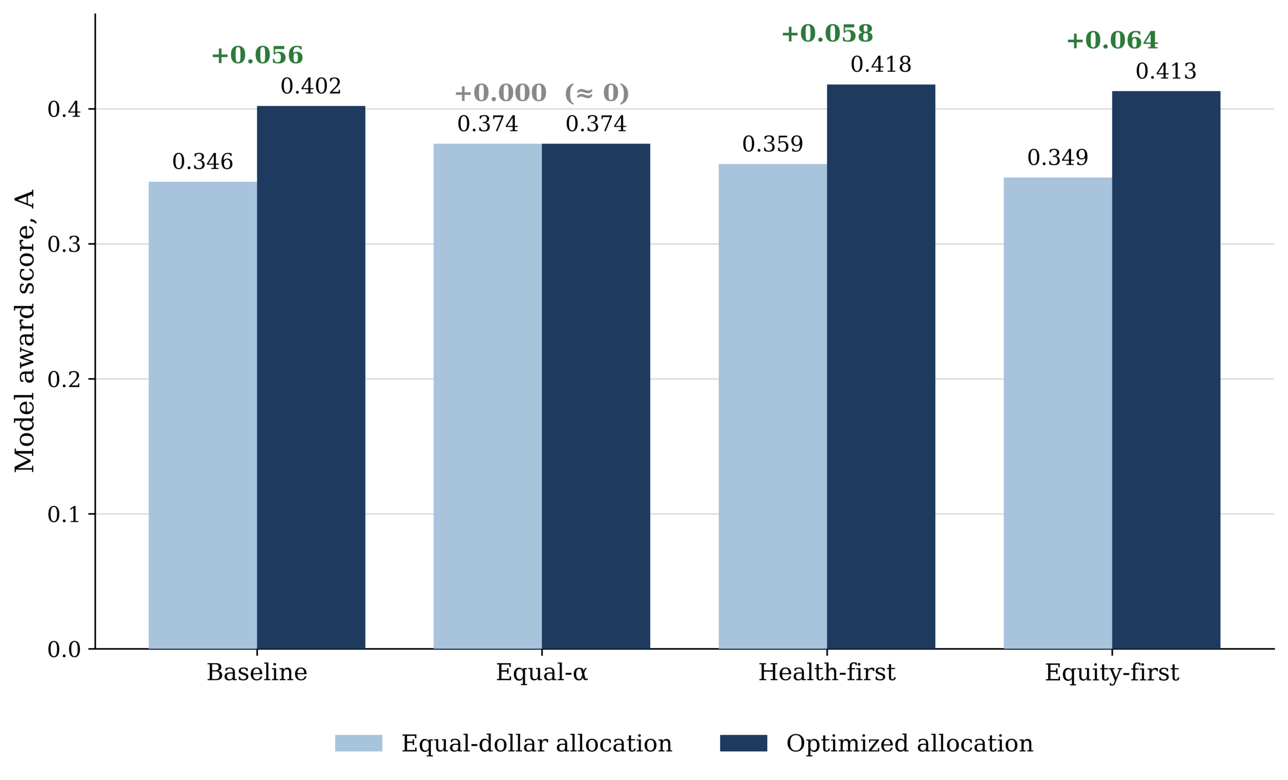
Four different policy weighting scenarios were tested to examine the robustness of the optimization approach and sensitivity of the societal benefit index to the weighting of policies. It should be emphasized at the outset that the dominance of optimized over uniform allocation is not merely an empirical regularity observed across these particular scenarios; it follows directly from optimizing a concave award function, though its magnitude depends on the heterogeneity of the α weights. The scenarios below therefore serve to illustrate the magnitude and distribution of this gain under different policy priorities. The index values are not strictly comparable across scenarios because each scenario has a different set of α weights; the cross-scenario comparisons below are descriptive, showing which set of priorities attains the highest score under its own weighting. Figure 1 summarizes the resulting societal benefit index values for each scenario, and Table 5 reports the underlying allocations.

Scenario	Public Safety ($M)	Health ($M)	Social Services ($M)	Schools ($M)	Econ. Dev. ($M)	Equal-dollar A	Total Award A
Baseline	$2.29	$3.39	$3.15	$14.10	$0.24	0.346	0.402
Equal α	$4.71	$4.81	$4.74	$4.55	$4.36	0.374	0.374
Health-first	$1.67	$14.36	$5.53	$0.71	$0.90	0.359	0.418
Equity-first	$2.33	$3.46	$15.18	$1.96	$0.24	0.349	0.413

Note: Each scenario’s Total Award A is compared against its own Equal-dollar A. The equal-dollar A is the uniform-share allocation scored under that scenario’s own α and β. β values are held constant across scenarios. All scenarios use the optimization procedure described in the Optimization Procedure section.

For all four optimized scenarios, uniform allocation is matched or outperformed. The baseline model (A = 0.402) results in a gain of +0.056 compared to uniform, with the bulk of the gain going to schools. The smallest gain (approximately 0.000) is expected from the equal α model (A = 0.374) since equal weights place the optimum almost exactly at the equal-dollar split, leaving little room for β differences to improve the allocation. Additionally, the health-first model (A = 0.418) has the highest index of benefit to society of all the models, with +0.058 over uniform. This is due to the high β for health (0.65) and its high α weight (0.35), leading to a large marginal return at concentrated allocation levels. Lastly, the equity-first model (A = 0.413) delivers the second-highest societal benefit index overall and the largest gain over its equal-dollar baseline (+0.064), with 65.5% of the surplus allocated to social services. The relatively high β of social services results in an index value that is closer to the health-first scenario. To quantify how concentrated each allocation is, the Herfindahl–Hirschman Index (HHI) and Gini coefficient were computed across the five domain shares reported in Table 5; the results are given in Table 6. Both confirm that the optimized scenarios concentrate surplus far more than uniform allocation, making explicit the efficiency–concentration relationship discussed above.

Scenario	HHI	Gini
Uniform (flat)	2,000	0.000
Baseline	4,201	0.498
Equal α	2,002	0.019
Health-first	4,487	0.551
Equity-first	4,689	0.542

Note: HHI = Herfindahl–Hirschman Index (sum of squared percentage shares; 2,000 = even five-way split, 10,000 = all surplus to one domain). Gini = Gini coefficient across domains (0 = perfectly even, 0.8 = maximum for five domains). Both measure domain-level concentration, not social equity. Values computed from Table 5 allocations.

Optimization Dominance

In all of the weighting scenarios the optimized allocation matches or outperforms the uniform distribution by up to 0.064. The size of the net gain largely depends on the heterogeneity of the α weights; it is large when priorities differ across domains and negligible when they are equal. The mathematical explanation for this is that the optimum allocation reallocates resources from less productive domains towards more productive ones until the marginal awards are equalized, and that is valid for all domains because of the fact that β < 1 for all domains. Finally, the result demonstrates that the use of evidence-based optimization for selecting the allocation of surplus yields a higher value of the benefit index for the society as a whole, though its size depends on the Board’s priorities.

The qualitative results are robust to parameter perturbation: In the Monte Carlo analysis, the schools’ allocation was the largest in 100.0% of the 10,000 draws, with a median allocation of 59.8% (90% interval: 43.2% to 75.1%) and the gain over the scenario’s own equal-dollar baseline was positive in every draw (median 0.060; minimum 0.022). The two qualitative findings of the study are not dependent on the actual percentages assigned to the parameters, but rather on their ordering.

Discussion

The Equity-Efficiency Tradeoff in Optimized Allocation

In terms of the two research questions, the results illustrate that optimized allocation is either equal to or better than each scenario’s equal-dollar baseline, and that the health-first weighting generates the highest index value, followed by equity-first. While uniform allocation might seem fair in that it gives each domain an equal amount, it would result in a lower value of the societal benefit index. Under optimized allocation, the amount of resources allocated in higher return domains (mainly schools) raises the overall index value while reducing the value of the four other domains. This tension mirrors Okun’s insight that the quest for equality often comes at a cost to efficiency, and that there is a basic tradeoff between equality and efficiency in society⁶⁵. However, it is important to acknowledge that the current results point to the fact that this tradeoff may not be as strong as Okun’s formulation would suggest in the case of public investment. In the U.S. context, Meier et al. present results of citizen experiments that test the effectiveness-equity-efficiency tradeoff in K-12 education programs and reveal that citizens value both effectiveness and equity, and are not willing to sacrifice one for the sake of the other, implying that there are significant limitations for policy makers when attempting to make efficiency-maximizing allocations⁶⁶. The award function operationalizes the framework and gives the policymaker the flexibility to determine the equity-efficiency trade-off, rather than the implicit equity of one-size-fits-all. This can especially be seen in the equity-first scenario, with A = 0.413. In this case, the largest α weight was moved to social services (0.35), and the scenario resulted in a higher societal benefit index value than the uniform allocation scenario – 65.5% of the surplus going to the domain serving the most economically vulnerable populations. The conclusion we can draw, then, is that the priorities of equity are not at odds with optimization but rather they yield another optimal allocation which is still better than the flat allocation. A related concern is that the optimization operates on surplus shares without reference to domains’ very different existing budgets: public safety’s 9.9% share ($2.29M against a $704M budget) and FCPS’s 60.9% ($14.10M against $3,052M) represent much closer proportional increments (0.33% versus 0.46%). This is a deliberate consequence of the share-based formulation (discussed under the share-based formulation in the Methods), which was chosen over a budget-relative formula that awarded disproportionate surplus to small-budget domains. The cost is that the model does not capture how a dollar addition interacts with a domain’s existing scale – a limitation discussed further under scale invariance below.

Implementation Barriers in Evidence-Based Budgeting

While the mathematical results consistently show that optimized allocation matches or outperforms uniform allocation across the tested weighting scenarios, the practical implementation of this evidence-based budgeting faces significant institutional barriers. For example, 76% of state and local government leaders surveyed by the Pew Charitable Trusts said that data-driven decision-making is a significant challenge, and less than half felt that their staff were sufficiently trained to make data-driven decisions. Pew also notes that incremental budgeting is built into the policy structure, making it a barrier to evidence-based allocation⁶⁷. The National League of Cities and Government Finance Officers Association similarly surveyed municipal officials, including mayors, city managers, and staff (138 respondents), and found that over half identified difficulties in connecting the budget line items to organizational goals and a lack of elected official knowledge of budgeting as major barriers to evidence-based allocation⁶⁸. To combat this, the award function requires only two parameters per domain (α and β), both of which can be derived from existing published research without original data collection or econometric estimation. The scenario analysis framework allows policymakers to explore multiple configurations without committing to a single set of weights, which reduces the political risk of adopting a quantitative framework. Nevertheless, the real challenge lies in the institutional barrier that is described by Raudla: politicians tend to make limited use of performance information in the budget process⁶⁹. The award function provides the analytical infrastructure for this shift; however, its adoption depends on the political will and organization capacity that lie beyond the scope of mathematical optimization.

The Scale Invariance Problem

One notable property of the share-based formulation (s_i/S) is that the optimal allocation shares are invariant to the level of surplus S. Whether the Board allocates $23.17 million or $230 million, the model recommends the same percentage distribution: 60.9% to schools, 14.6% to health, and so on. While this property is mathematically convenient in terms of ensuring that the model’s recommendations are robust to changes in available surplus, it also represents a limitation. This can largely be attributed to the fact that the returns on public spending are likely to exhibit threshold effects that a share-based model cannot capture. A $14 million increase in FCPS funding may produce different marginal returns than a $140 million increase, as the former could fund additional teaching positions, compared to the latter, which could enable systemic infrastructure improvements with potentially nonlinear returns. Pritchett and Filmer revealed that the productivity of education spending depends heavily on which inputs the money purchases, suggesting that aggregate spending elasticities may not be stable across contexts or spending levels⁷⁰. Future work could build on this model by incorporating a budget-relative component or piecewise-linear approximations of the award function at different surplus scales to address this. There is also an absorptive-capacity concern at high surpluses, because of this scale invariance. When the recommended shares are fixed, a much larger surplus (e.g., $500M) would direct 60.9% – approximately $304M – to FCPS in one year, an amount the division may not be able to use productively, which would in turn violate the diminishing-returns premise upon which the model is based. One natural extension is to add upper-bound constraints on the amount of each domain that can be absorbed in any given year, with the surplus at the upper bound being moved to another domain.

Conclusion and Future Directions

This study developed and applied an award function optimization model to the allocation of $23.17 million in discretionary budget surplus in Fairfax County, Virginia. The model is based on the Cobb-Douglas production function⁵⁷, the Bergson-Samuelson social welfare framework^61,62 and the public expenditure composition literature⁶. Moreover, its parameters are calibrated to Fairfax County using evidence from peer-reviewed research in education economics, public health, public safety, social services, and economic development. The main result of the paper is that the evidence-based optimization matches or outperforms uniform allocation by up to 0.064 on the societal benefit index under all four optimized weighting scenarios considered, showing robustness to policy weighting. Furthermore, two allocation strategies are presented: First, a baseline allocation strategy that allocates 60.9% of surplus to schools, reflecting the gap caused by the underfunding of the FCPS; and second, a health-first allocation strategy that maximizes the societal benefit index (0.418). The allocations are not prescriptions because the parameters are evidence-based and not locally estimated and the model does not include cross-domain complementarities and parameter uncertainty. Future research should continue to estimate elasticities for counties based on local administrative data and use this model with the parameters associated with it. Adding more cross-domain complementarities (specifically between health and social services) to the model and testing the results of the model for generalizability in other jurisdictions beyond Fairfax County will be key to explore in the future. A complementary validation would retrospectively test the model for several years of expenditure data from Fairfax County and see if the historical expenditure allocations between years were in line with the direction of the model output. If they prove to be consistent, this provides empirical support for the parametrization. Conversely, if they diverge, it would highlight areas where the parameters used in the literature do not seem to correlate well with the historical conditions in Fairfax County. Finally, a longitudinal study which contrasted the allocations in the model with the actual results of the budget would constitute the most direct test of the validity of the award function as a budget policy.

Acknowledgements

The author thanks the Fairfax County Department of Management and Budget for making FY 2027 budget documents publicly available.

Supplementary Material

References

1. V. Tanzi, L. Schuknecht. Public Spending in the 20th Century: A Global Perspective. Cambridge University Press, 2000. https://doi.org/10.1017/CBO9780511625800. [↩]
2. A. Afonso, L. Schuknecht, V. Tanzi. Public sector efficiency: an international comparison. Public Choice. Vol. 123, pg. 321–347, 2005, https://doi.org/10.1007/s11127-005-7165-2. [↩]
3. OECD. Government at a Glance 2015. OECD Publishing, 2015. https://doi.org/10.1787/gov_glance-2015-en. [↩]
4. R. J. Barro. Government spending in a simple model of endogenous growth. Journal of Political Economy. Vol. 98, pg. S103–S125, 1990, https://doi.org/10.1086/261726. [↩] [↩] [↩] [↩] [↩]
5. R. Kneller, M. F. Bleaney, N. Gemmell. Fiscal policy and growth: evidence from OECD countries. Journal of Public Economics. Vol. 74, pg. 171–190, 1999, https://doi.org/10.1016/S0047-2727(99)00022-5. [↩] [↩]
6. S. Devarajan, V. Swaroop, H. Zou. The composition of public expenditure and economic growth. Journal of Monetary Economics. Vol. 37, pg. 313–344, 1996, https://doi.org/10.1016/S0304-3932(96)90039-2. [↩] [↩] [↩] [↩] [↩] [↩]
7. C. K. Jackson, C. L. Mackevicius. What impacts can we expect from school spending policy? Evidence from evaluations in the United States. American Economic Journal: Applied Economics. Vol. 16, pg. 412–446, 2024, https://doi.org/10.1257/app.20220279. [↩] [↩] [↩]
8. J. Lafortune, J. Rothstein, D. W. Schanzenbach. School finance reform and the distribution of student achievement. American Economic Journal: Applied Economics. Vol. 10, pg. 1–26, 2018, https://doi.org/10.1257/app.20160567. [↩] [↩] [↩]
9. R. Masters, E. Anwar, B. Collins, R. Cookson, S. Capewell. Return on investment of public health interventions: a systematic review. Journal of Epidemiology and Community Health. Vol. 71, pg. 827–834, 2017, https://doi.org/10.1136/jech-2016-208141. [↩] [↩] [↩] [↩]
10. G. P. Mays, S. A. Smith. Evidence links increases in public health spending to declines in preventable deaths. Health Affairs. Vol. 30, pg. 1585–1593, 2011, https://doi.org/10.1377/hlthaff.2011.0196. [↩] [↩] [↩] [↩]
11. A. Chalfin, J. McCrary. Are U.S. cities underpoliced? Theory and evidence. Review of Economics and Statistics. Vol. 100, pg. 167–186, 2018, https://doi.org/10.1162/REST_a_00694. [↩] [↩] [↩] [↩] [↩] [↩]
12. S. Mello. More cops, less crime. Journal of Public Economics. Vol. 172, pg. 174–200, 2019, https://doi.org/10.1016/j.jpubeco.2018.12.003. [↩] [↩] [↩]
13. D. N. Hyman. Public finance: a contemporary application of theory to policy. Cengage Learning, 2014. [↩]
14. A. B. Wildavsky, N. Caiden. The new politics of the budgetary process. Pearson Longman, 2003. [↩]
15. I. S. Rubin. The politics of public budgeting. CQ Press, 2019. [↩]
16. U.S. Census Bureau. 2024 American Community Survey 1-year estimates. https://data.census.gov/ 2025. [↩] [↩]
17. Fairfax County Department of Management and Budget. FY 2027 advertised budget plan: Overview and Volume 1—General Fund. https://www.fairfaxcounty.gov/budget/sites/budget/files/Assets/documents/fy2027/advertised/overview.pdf 2026. [↩] [↩] [↩] [↩] [↩] [↩] [↩] [↩] [↩]
18. Joint Legislative Audit and Review Commission. Virginia’s K–12 funding formula. https://jlarc.virginia.gov/landing-2023-virginias-k-12-funding-formula.asp 2023. [↩] [↩]
19. Fairfax County Public Schools. FY 2025 approved budget. https://www.fcps.edu/sites/default/files/media/pdf/FY-2025-Approved-Budget.pdf 2024. [↩] [↩] [↩] [↩]
20. Fairfax County Government. Federal government resource hub. https://www.fairfaxcounty.gov/topics/federal-government-resource-hub 2026. [↩]
21. S. Boyd, L. Vandenberghe. Convex optimization. Cambridge University Press, 2004. [↩] [↩] [↩] [↩]
22. J. S. Coleman. Equality of educational opportunity. Equity & Excellence in Education. Vol. 6, pg. 19–28, 1968, https://doi.org/10.1080/0020486680060504. [↩]
23. E. A. Hanushek. The failure of input‐based schooling policies. The Economic Journal. Vol. 113, pg. F64–F98, 2003, https://doi.org/10.1111/1468-0297.00099. [↩]
24. E. A. Hanushek. Assessing the effects of school resources on student performance: an update. Educational Evaluation and Policy Analysis. Vol. 19, pg. 141–164, 1997, https://doi.org/10.3102/01623737019002141. [↩]
25. E. A. Hanushek, L. Woessmann. The economics of international differences in educational achievement. in Handbook of the Economics of Education Vol. 3 pg. 89–200, Elsevier, 2011. https://doi.org/10.1016/B978-0-444-53429-3.00002-8. [↩]
26. C. K. Jackson, R. C. Johnson, C. Persico. The effects of school spending on educational and economic outcomes: evidence from school finance reforms. The Quarterly Journal of Economics. Vol. 131, pg. 157–218, 2016, https://doi.org/10.1093/qje/qjv036. [↩] [↩] [↩] [↩] [↩] [↩] [↩]
27. B. D. Baker, D. Knight. Does money matter in education? https://www.shankerinstitute.org/resource/does-money-matter-in-education 2025. [↩]
28. D. Allen, R. Reich. Education, Justice, and Democracy. University of Chicago Press, 2013. https://doi.org/10.7208/chicago/9780226012933.001.0001. [↩]
29. E. J. Baron. School spending and student outcomes: evidence from revenue limit elections in Wisconsin. American Economic Journal: Economic Policy. Vol. 14, pg. 1–39, 2022, https://doi.org/10.1257/pol.20200226. [↩] [↩]
30. J. Rothstein, D. W. Schanzenbach. Does money still matter? attainment and earnings effects of post-1990 school finance reforms. Journal of Labor Economics. Vol. 40, pg. S141–S178, 2022, https://doi.org/10.1086/717934. [↩]
31. E. Rauscher, Y. Shen. Variation in the relationship between school spending and achievement: progressive spending is efficient. American Journal of Sociology. Vol. 128, pg. 189–223, 2022, https://doi.org/10.1086/719956. [↩]
32. D. Card, A. A. Payne. School finance reform, the distribution of school spending, and the distribution of student test scores. Journal of Public Economics. Vol. 83, pg. 49–82, 2002, https://doi.org/10.1016/S0047-2727(00)00177-8. [↩]
33. Z. Lindenfeld, A. I. Mauri, J. E. Chang. Examining the relationship between local governmental expenditures on the social determinants of health and county-level overdose deaths, 2017-2020. Journal of Public Health Management & Practice. Vol. 31, pg. 20–28, 2025, https://doi.org/10.1097/PHH.0000000000001983. [↩]
34. S. J. Sowmyan, A. H. Hirai, J. S. Kaufman. State and local government expenditures and infant mortality. Pediatrics. Vol. 154, pg. e2023063571, 2024, https://doi.org/10.1542/peds.2023-063571. [↩]
35. S. R. Singh. Public health spending and population health. American Journal of Preventive Medicine. Vol. 47, pg. 634–640, 2014, https://doi.org/10.1016/j.amepre.2014.05.017. [↩]
36. J. P. Leider, N. Alfonso, B. Resnick, E. Brady, J. M. McCullough, D. Bishai. Assessing the value of 40 years of local public expenditures on health. Health Affairs. Vol. 37, pg. 560–569, 2018, https://doi.org/10.1377/hlthaff.2017.1171. [↩]
37. H. C. Turner, Y. Hori, P. Revill, W. Rattanavipapong, K. Arai, J. Nonvignon, M. Jit, Y. Teerawattananon. Analyses of the return on investment of public health interventions: a scoping review and recommendations for future studies. BMJ Global Health. Vol. 8, pg. e012798, 2023, https://doi.org/10.1136/bmjgh-2023-012798. [↩]
38. B. Bekemeier, D. Grembowski, Y. R. Yang, J. R. Herting. Local public health delivery of maternal child health services: are specific activities associated with reductions in Black–White mortality disparities? Maternal and Child Health Journal. Vol. 16, pg. 615–623, 2012, https://doi.org/10.1007/s10995-011-0794-9. [↩]
39. W. N. Evans, E. G. Owens. COPS and crime. Journal of Public Economics. Vol. 91, pg. 181–201, 2007, https://doi.org/10.1016/j.jpubeco.2006.05.014. [↩]
40. Y. Lee, J. E. Eck, N. Corsaro. Conclusions from the history of research into the effects of police force size on crime—1968 through 2013: a historical systematic review. Journal of Experimental Criminology. Vol. 12, pg. 431–451, 2016, https://doi.org/10.1007/s11292-016-9269-8. [↩]
41. E. L. Piza, V. F. Chillar. The effect of police layoffs on crime: a natural experiment involving New Jersey’s two largest cities. Justice Evaluation Journal. Vol. 4, pg. 176–196, 2021, https://doi.org/10.1080/24751979.2020.1858697. [↩]
42. C. I. A. Oronce, N. A. Ponce, C. A. Sarkisian, F. J. Zimmerman, Y. Tsugawa. Association between governmental spending on social services and health care use among low-income older adults. Health Affairs Scholar. Vol. 3, pg. qxae181, 2025, https://doi.org/10.1093/haschl/qxae181. [↩]
43. E. H. Bradley, M. Canavan, E. Rogan, K. Talbert-Slagle, C. Ndumele, L. Taylor, L. A. Curry. Variation in health outcomes: the role of spending on social services, public health, and health care, 2000–09. Health Affairs. Vol. 35, pg. 760–768, 2016, https://doi.org/10.1377/hlthaff.2015.0814. [↩] [↩] [↩]
44. C. Cardona, N. S. Anand, Y. N. Alfonso, J. P. Leider, J. M. McCullough, B. Resnick, D. Bishai. County health outcomes linkage to county spending on social services, building infrastructure, and law and order. SSM – Population Health. Vol. 16, pg. 100930, 2021, https://doi.org/10.1016/j.ssmph.2021.100930. [↩]
45. D. J. Elgin, M. Kluckman, H. Ringeisen, M. Dolan. National Survey of Child and Adolescent Well-Being III workforce study: reasons for child welfare caseworker turnover from 2021 to 2022. https://acf.gov/opre/report/national-survey-child-and-adolescent-well-being-iii-workforce-study-reasons-child 2025. [↩] [↩] [↩]
46. E. Lee, K. Kirkland, C. Miranda-Julian, R. Greene. Reducing maltreatment recurrence through home visitation: a promising intervention for child welfare involved families. Child Abuse & Neglect. Vol. 86, pg. 55–66, 2018, https://doi.org/10.1016/j.chiabu.2018.09.004. [↩] [↩] [↩]
47. P. J. Fowler, D. Chavira. Family unification program: housing services for homeless child welfare–involved families. Housing Policy Debate. Vol. 24, pg. 802–814, 2014, https://doi.org/10.1080/10511482.2014.881902. [↩]
48. T. Bartik. Making Sense of Incentives: Taming Business Incentives to Promote Prosperity. W.E. Upjohn Institute, 2019. https://doi.org/10.17848/9780880996693. [↩] [↩] [↩]
49. D. A. Kenyon, A. H. Langley, B. P. Paquin. Rethinking property tax incentives for business. Lincoln Institute of Land Policy, 2012. [↩] [↩]
50. E. Glaeser. Triumph of the city: how our greatest invention makes us richer, smarter, greener, healthier, and happier. Penguin Books, 2011. [↩] [↩] [↩]
51. E. Moretti. The new geography of jobs. Houghton Mifflin Harcourt, 2012. [↩] [↩]
52. A. Afonso, D. Furceri. Government size, composition, volatility and economic growth. European Journal of Political Economy. Vol. 26, pg. 517–532, 2010, https://doi.org/10.1016/j.ejpoleco.2010.02.002. [↩]
53. R. K. Armey. The freedom revolution: the new Republican House majority leader tells why big government failed, why freedom works, and how we will rebuild America. Regnery Publishing, 1995. [↩]
54. O. F. Altunc, C. Aydın. The relationship between optimal size of government and economic growth: empirical evidence from Turkey, Romania and Bulgaria. Procedia – Social and Behavioral Sciences. Vol. 92, pg. 66–75, 2013, https://doi.org/10.1016/j.sbspro.2013.08.639. [↩]
55. M. Kolçak, A. Y. Kalabak. Do government expenditures subject to law of diminishing returns? A panel data application. in Proceedings of the International Conference on Eurasian Economies, pg. 249–256, Tashkent, Uzbekistan, 2018. https://doi.org/10.36880/C10.02212. [↩]
56. United Nations Conference on Trade and Development. The costs of achieving the SDGs: methodology. https://unctad.org/sdg-costing/methodology 2024. [↩]
57. C. W. Cobb, P. H. Douglas. A theory of production. The American Economic Review. Vol. 18, pg. 139–165, 1928. [↩] [↩]
58. R. M. Solow. A contribution to the theory of economic growth. The Quarterly Journal of Economics. Vol. 70, pg. 65–94, 1956, https://doi.org/10.2307/1884513. [↩]
59. H. R. Varian. Intermediate microeconomics: a modern approach. W.W. Norton & Company, 2014. [↩]
60. T. J. Galama, P. Hullegie, E. Meijer, S. Outcault. Is there empirical evidence for decreasing returns to scale in a health capital model? Health Economics. Vol. 21, pg. 1080–1100, 2012, https://doi.org/10.1002/hec.2843. [↩]
61. A. Bergson. A reformulation of certain aspects of welfare economics. The Quarterly Journal of Economics. Vol. 52, pg. 310–334, 1938, https://doi.org/10.2307/1881737. [↩] [↩]
62. P. A. Samuelson. Foundations of economic analysis. Harvard University Press, 1947. [↩] [↩]
63. M. D. Adler. Measuring social welfare: an introduction. Oxford University Press, 2019. [↩]
64. S. Arslanalp, F. Bornhorst, S. Gupta, E. Sze. Public capital and growth. IMF Working Paper WP/10/175, International Monetary Fund, 2010. [↩]
65. A. M. Okun. Equality and efficiency: the big tradeoff. Brookings Institution Press, 1975. [↩]
66. K. J. Meier, J. Davis, X. Xu. Effectiveness, efficiency, and equity tradeoffs in public programs: a citizen experiment. Public Administration Review. Vol. 83, pg. 1462–1477, 2023, https://doi.org/10.1111/puar.13690. [↩]
67. Pew Charitable Trusts. A guide to evidence-based budget development. https://www.pewtrusts.org/en/research-and-analysis/issue-briefs/2016/07/a-guide-to-evidence-based-budget-development 2016. [↩]
68. National League of Cities & Government Finance Officers Association. Priorities, barriers & opportunities in the municipal budgeting process. https://www.nlc.org/article/2025/04/29/priorities-barriers-opportunities-in-the-municipal-budgeting-process/ 2025. [↩]
69. R. Raudla. Politicians’ use of performance information in the budget process. Public Money & Management. Vol. 42, pg. 144–151, 2022, https://doi.org/10.1080/09540962.2021.1989779. [↩]
70. L. Pritchett, D. Filmer. What education production functions really show: a positive theory of education expenditures. Economics of Education Review. Vol. 18, pg. 223–239, 1999, https://doi.org/10.1016/S0272-7757(98)00034-X. [↩]