A Variational Quantum Framework for the One-Dimensional Gross–Pitaevskii–Poisson Equation: Capabilities and Limitations

Abstract

Wave-like models of dark matter, described by the Gross–Pitaevskii–Poisson (GPP) equation, are expensive to simulate classically at high resolution, which has motivated interest in quantum approaches. In this work we ask a focused question: can a shallow variational quantum algorithm reproduce the basic dynamics of the 1D GPP equation? We implement a hardware-efficient variational circuit and an implicit, residual-based time-stepping scheme, and we evaluate it directly against a classical split-step Fourier solver for the same system. All simulations are exact statevector emulations run on a classical simulator; no quantum hardware and no finite-shot sampling are involved. We report three findings. First, the classical baseline reproduces the expected physics, forming smooth density cores whose sharpness is controlled by the self-interaction. Second, a variational circuit can prepare the physical initial state to a fidelity of 0.9995, so state preparation on this class of circuits is tractable. Third, the variational time-evolution scheme does not reproduce the dynamics: the original formulation consistently converges to a boundary-localized solution rather than the physical core, and even after correcting the equation and normalization the evolved state drifts from the physical solution with a relative error of order 100%. We conclude that faithful variational time evolution of this nonlinear, self-gravitating system requires a more principled approach, and we identify this as the direction for future work. This is a proof-of-concept and methods study rather than a demonstration of a working quantum simulation.

Keywords: dark matter; Gross–Pitaevskii–Poisson equation; variational quantum algorithm; quantum simulation; solitonic cores; state preparation

Introduction

Dark Matter and Wave Dark Matter

Dark matter makes up most of the matter in the universe, yet its nature remains unknown. It emits and absorbs no light, and is inferred only through its gravitational effects on the motion of galaxies and the growth of cosmic structure. Explaining that behaviour is one of the central open problems in physics.

For decades the standard approach has treated dark matter as a collection of particles interacting through gravity, simulated with classical N-body methods. These reproduce large-scale structure well but run into difficulty on galactic scales¹. One alternative is wave-like dark matter, in which a quantum wavefunction replaces point particles^2,3. The simplest such model uses the Schrödinger–Poisson equation, combining quantum pressure with gravity^4,5,6. Adding a self-interaction term produces the Gross–Pitaevskii–Poisson (GPP) equation, which can smooth the sharp density spikes that the simpler model tends to form^7,8,9.

Why Quantum Computing?

Solving these equations accurately is computationally demanding. The wavefunction must be resolved finely in space and evolved over long times, and the memory required grows quickly as the resolution increases. This is what motivates looking at quantum computing. Why might a quantum computer help simulate a wave equation? Because a quantum computer stores its information in qubits, which hold a quantum state directly: a wavefunction sampled on N grid points can in principle be encoded in only log₂N qubits, so a representation that becomes expensive on a classical grid can be held compactly, and quantum operations can evolve it. The object we want to simulate is, in this sense, the same kind of object a quantum computer natively manipulates.

Variational Quantum Algorithms

Why, then, can we not simply run this on today’s quantum computers? Current devices are in the noisy intermediate-scale quantum (NISQ) era: they have a limited number of qubits, and every gate introduces a small error, so those errors accumulate and deep circuits quickly become unreliable^10,11. A full, exact quantum evolution of our problem would require circuits far deeper than present hardware can run faithfully.

This constraint is what makes a variational quantum algorithm (VQA) a sensible choice. A VQA pairs a shallow, parameterized quantum circuit with a classical optimizer: the circuit prepares a trial wavefunction, a cost function measures how far that state is from satisfying the target equations, and the optimizer adjusts the circuit’s parameters to reduce the cost^12,13,14. Because the quantum circuit stays shallow, a VQA is one of the few strategies suited to near-term hardware.

VQAs are not the only quantum route to such problems. Other proposals include Hamiltonian-simulation methods based on Trotterization¹⁵ and linear-systems or block-encoding approaches¹⁶, often combined with Carleman linearization to handle the nonlinear term^17,18,19. The specific variational method we use builds on Lubasch et al.²⁰, who solved nonlinear problems including the nonlinear Schrödinger equation variationally, and on Mocz and Szasz²¹, who applied a variational approach to the Schrödinger–Poisson system.

Research Question and Contributions

This paper investigates whether a shallow variational quantum algorithm can reproduce the dynamics of the one-dimensional Gross–Pitaevskii–Poisson equation. This work makes three contributions. First, it extends the variational framework of Mocz and Szasz²¹ to include the GPP self-interaction term. Second, it benchmarks the method quantitatively against a classical split-step Fourier solver rather than by visual inspection alone. Third, it identifies the principal limitation of the present implementation, showing that state preparation succeeds while variational time evolution remains the dominant source of error.

Background

This section briefly introduces the concepts used later. The Gross–Pitaevskii–Poisson equation is a model of a self-gravitating quantum wave: a single complex wavefunction feels its own gravity, spreads under quantum pressure, and pushes on itself through a self-interaction term whose sign can make the wave concentrate or disperse. Statevector simulation means computing the full complex quantum state exactly on a classical computer, without sampling measurement outcomes; it lets us study the algorithm’s behaviour with no hardware noise. Fidelity measures how close two quantum states are, equal to one when they are identical; we use it to quantify how well the circuit prepares a target state. The relative L² error measures the normalized difference between two density profiles; we use it to compare the variational output against the classical baseline.

Methods

Gross–Pitaevskii–Poisson Equation

We study wave-like dark matter in one dimension. In dimensionless form the wavefunction obeys

and the gravitational potential is fixed by the Poisson equation sourced by the density fluctuation,

Each term has a clear physical meaning. The time-evolution term i∂_tψ describes how the wavefunction changes in time; the factor i gives the standard form of quantum evolution and conserves the total mass. The quantum-pressure term −½∇²ψ arises from the curvature of the wavefunction and produces a dispersive effect that resists gravitational collapse and smooths the density. The gravitational term Vψ couples the wave to the potential sourced by its own density, pulling matter toward overdense regions. The self-interaction term g|ψ|²ψ sets how the wave acts on itself: for g > 0 it is repulsive, smoothing the density and producing broader cores; for g = 0 it vanishes, recovering the Schrödinger–Poisson model; and for g < 0 it is attractive, concentrating the density and sharpening peaks²².

The density is ρ = |ψ|², normalized so that its mean value is one. With this convention the Poisson source ρ − 1 has zero mean, which is the condition required for the periodic Poisson equation to have a solution. All simulations use a periodic domain of length L = 8, discretized on a uniform grid of N = 2ⁿ points, where n is the number of qubits. The initial condition is the smooth density wave

renormalized to unit mean density; its peak sits at x = 2.

Computational Scope

Every result reported here is an exact statevector emulation carried out on a classical simulator, using PennyLane’s default.qubit statevector device. No physical quantum hardware was used, and no finite-shot measurement sampling was performed: the full complex state vector is available at every step. Consequently this study makes no claims about hardware performance or noise resilience; a finite-shot, hardware-noise study is left as future work. Because the circuit state is always exactly unit-normalized, the physical field is taken as φ = √N ψ, so that ρ = |φ|² = N|ψ|² has unit mean by construction. This is a one-dimensional, proof-of-concept study.

Variational Quantum Circuit

The wavefunction is represented by a layered, hardware-efficient circuit²³. Each layer applies a single-qubit RY rotation and a single-qubit RZ rotation to every qubit, followed by a chain of CNOT gates between neighbouring qubits. The rotations set the amplitude and phase of each qubit, while the CNOT gates entangle adjacent qubits, together allowing the circuit to represent interference and spatial correlations in the wavefunction. The number of layers, the circuit depth, is fixed at n−1. Deeper circuits can represent more complex states but accumulate more noise on real hardware, so the depth is kept shallow to reflect near-term constraints.

Cost Function and Optimization

The physics is encoded in two cost functions that measure how far the current state is from satisfying the governing equations; a classical optimizer minimizes them. The potential cost enforces the Poisson equation. On the grid the Laplacian is approximated by the standard three-point finite difference, ∇²V_i = (V_i−1 − 2V_i + V_i+1)/dx², and

where ρ = N|ψ|² and λ is a numerical weight balancing the relative scale of the two cost terms (set to 1 in most runs). The wavefunction cost advances the state in time; writing φ for the current physical field and φ′ for the updated one,

Parameters are updated with a gradient-based optimizer (Adagrad, step size 0.02; the state-preparation experiments use Adam, step size 0.05), with eight inner optimization steps per time step.

Time-Stepping Scheme

Because the right-hand side of the residual in Eq. (5) is evaluated on the updated state φ′ rather than the current state φ, this is an implicit (backward-Euler-type) update, not a forward-Euler step; it is solved as a nonlinear optimization over the circuit parameters at each step. Each step optimizes the potential first (with the wavefunction fixed) and then the wavefunction (using the updated potential), and the state is renormalized after each update by ψ → ψ/‖ψ‖. The full procedure is:

Prepare parameters so that circuit(theta) approximates psi(x,0)
for t = 1 ... Nt:
    rho <- N * |circuit(theta)|^2
    solve  d_xx V = rho - 1   for V     (spectral Poisson solve; V fixed)
    repeat (inner optimization, fixed number of steps):
        phi' = sqrt(N) * circuit(theta)
        minimize  residual(theta)  over theta   (implicit GPP residual, Eq. 5)
    renormalize state

Simulation Parameters

The run parameters are collected in Table 1.

Parameter	Value(s)
Qubits n	4–9 (main sweep); 5 for the comparisons here
Grid points N	2ⁿ
Domain L (periodic)	8.0
Circuit depth	n−1 layers
Time step Δt	0.05
Time steps Nₜ	200 (up to 300)
Poisson weight λ	1.0 (3.0 for one repulsive run)
Optimizer	Adagrad, step size 0.02
Inner steps per time step	8

Classical Baseline and Evaluation Metrics

To provide the ground truth, we solve the identical 1D GPP system with a standard classical method: a split-step (time-splitting) spectral scheme²⁴. The kinetic term is advanced in Fourier space and the potential and nonlinear terms in real space, with the Poisson equation solved spectrally at each step. Agreement between the variational output and this baseline is assessed qualitatively through the density profiles and quantitatively using the relative L² error and the location of the density peak. These metrics let us distinguish successful state preparation from successful time evolution.

Results

Classical Baseline

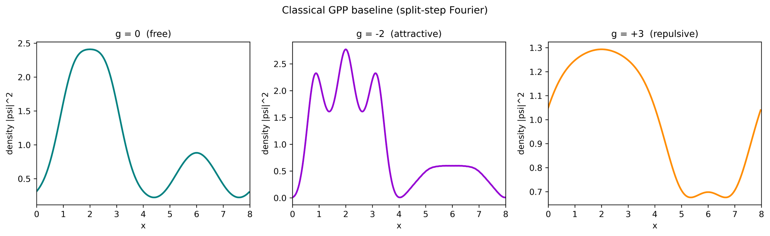
The classical baseline reproduces the expected physics of the GPP system (Figure 1). In all three regimes the density relaxes into a smooth, localized core centred near x = 2, the location of the initial overdensity. The self-interaction controls the sharpness of this core: the attractive case (g = −2) produces the most concentrated profile (peak density 2.77), the free case (g = 0) an intermediate one (2.41), and the repulsive case (g = +3) the flattest (1.29). The mean density is conserved at unity throughout. This ordering—sharper cores for attractive interactions, broader profiles for repulsive ones—is the physical behaviour the variational method is expected to reproduce.

Original Variational Algorithm

Run as originally formulated, the variational algorithm does not reproduce this behaviour (Figure 2). For every value of g, the output density concentrates almost entirely at the first grid point, x = 0: roughly 96% of the density sits at that single point. The three regimes produce essentially identical output—the attractive, free, and repulsive cases are indistinguishable—so the qualitative g-dependence is not present in the data. Against the baseline on a matched 32-point grid, the relative L² errors are large in all cases (Table 2).

Regime	VQA peak	Baseline peak	Relative L² error
g = 0	x = 0	x ≈ 2.1	438%
g = −2	x = 0	x ≈ 1.6	336%
g = +3	x = 0	x ≈ 2.1	521%

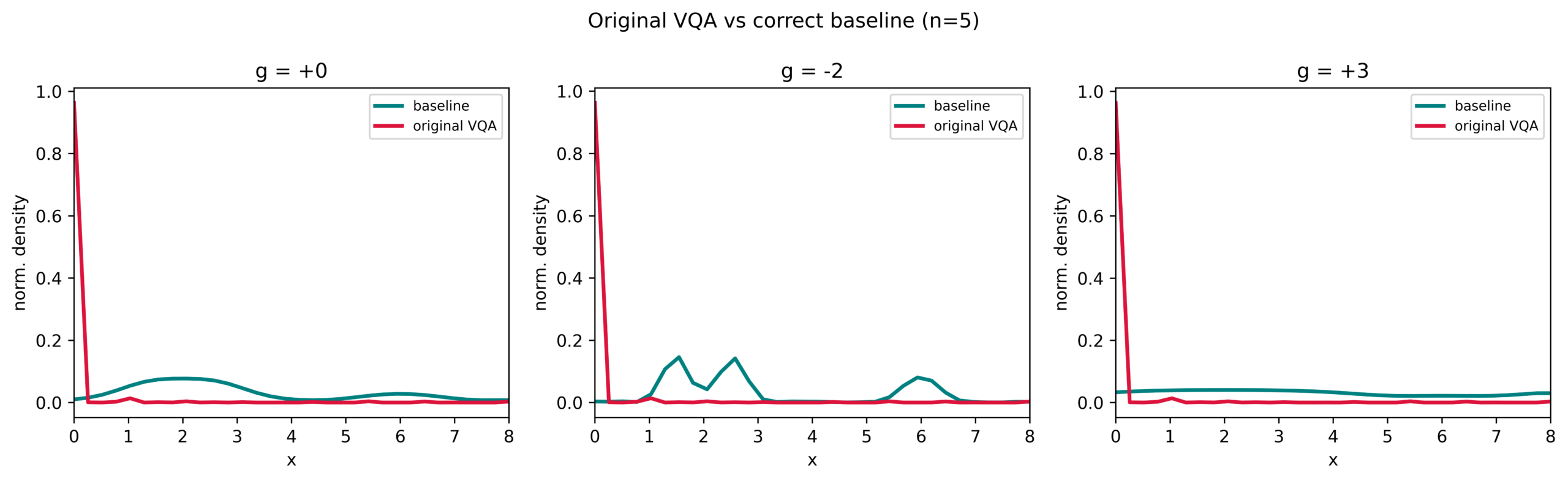
The original implementation deviated from the formulation above in three respects: the kinetic term carried the wrong coefficient and sign, the wavefunction was normalized to unit total probability rather than unit mean density (so the gravitational source ρ−1 was nearly constant and gravity had little effect), and the circuit was initialized with small random angles rather than at the physical state. The mechanism of the boundary pile-up then follows: a hardware-efficient circuit with small random rotation angles has an output dominated by the |0⋯0⟩ basis component, which corresponds to the first grid point. The implicit residual has this concentrated configuration as an approximate fixed point, and the optimization does not move away from it. The behaviour is fully established within the first few dozen steps and does not change with more steps, indicating a structural limitation rather than a convergence failure.

Corrected Implementation

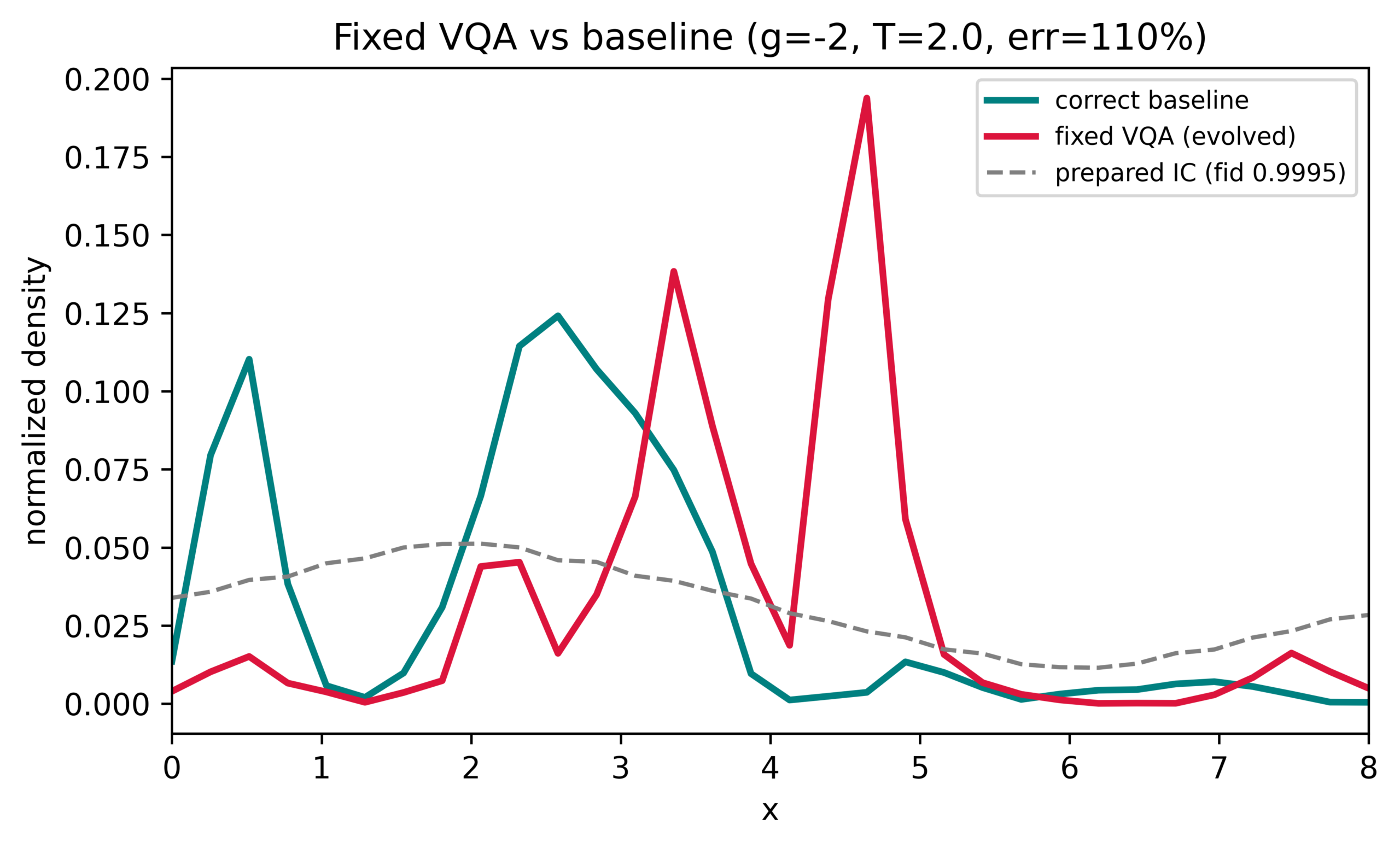
We next corrected the formulation—the −½ kinetic coefficient, the mean-density-one normalization, and the density definition ρ = N|ψ|²—and added an explicit variational state-preparation step in which the circuit is first trained to reproduce the physical initial wave before evolution begins. The two components behave very differently (Figure 3).

State preparation is successful: the circuit reproduces the initial density wave to a fidelity of 0.9995, with the prepared density correctly peaked at x = 2.06. A depth-(n−1) hardware-efficient circuit is therefore expressive enough to hold the physical state.

Time evolution is not successful. Starting from the prepared state and evolving with the corrected scheme, the density drifts away from the physical core. Depending on the optimizer and the number of inner steps, the peak migrates to x ≈ 0.8 or overshoots to x ≈ 4.6, with a relative L² error against the baseline of approximately 100% in both cases. Increasing the optimization per step does not reduce this error; it only changes the direction of the drift.

Comparative Analysis

Table 3 summarizes the comparison across methods.

Method	Density peak	Fidelity	Relative L² error
Original VQA (g = −2)	x = 0	—	336%
Corrected, prepared state	x = 2.06	0.9995	—
Corrected, after evolution	x ≈ 0.8 or 4.6	—	~100%
Classical baseline (g = −2)	x ≈ 1.6	—	reference

Discussion

The results separate cleanly into a success and a failure, and the contrast is informative. State preparation succeeds to 0.9995 fidelity, which shows that the shallow hardware-efficient circuit is expressive enough to represent the physical state; expressibility is therefore not the limiting factor. During time evolution, however, the state drifts away from the physical solution regardless of how hard each step is optimized. This points to the time-stepping procedure itself: minimizing a residual at each step does not, on its own, enforce the correct dynamics, and small errors accumulate into a systematic drift.

This is consistent with the surrounding literature. Mocz and Szasz²¹ reported qualitative agreement for the Schrödinger–Poisson system but without a quantitative comparison to a classical solver, so a drift of this kind could go unnoticed. More recent variational-time-evolution work uses more structured procedures—the multi-copy tensor-network approach of Lubasch et al.²⁰, the grid-based variational time evolution of Ollitrault et al.²⁵, and the evolution-equation solver of Leong et al.²⁶—rather than naive per-step residual minimization. Taken together, the evidence suggests that the principal bottleneck lies in the variational time-evolution procedure rather than in the expressibility of the circuit.

Several limitations bound these conclusions. The study is one-dimensional, uses a single hardware-efficient ansatz family, and is run entirely as an exact statevector emulation with no measurement noise; the behaviour on real hardware, and in higher dimensions, remains open.

Conclusion

We set out to test whether a shallow variational quantum algorithm could reproduce the dynamics of the 1D Gross–Pitaevskii–Poisson equation, evaluated against a classical baseline. The classical split-step baseline behaves as expected, forming smooth density cores whose sharpness tracks the sign and strength of the self-interaction. Against this reference, the variational method separates into two parts: state preparation is successful, reaching a fidelity of 0.9995, while time evolution is not, drifting from the physical solution by a relative error of order 100% that additional optimization does not remove.

The honest conclusion is that this variational scheme does not yet simulate the GPP system faithfully, and that the difficulty lies specifically in the time-evolution step rather than in representing the state. This is a useful negative result: it locates the bottleneck precisely and rules out initialization and expressibility as the causes.

Future Work

The natural next step is a more principled treatment of the time evolution. Residual minimization at each step does not enforce the correct dynamics reliably; a time-dependent variational principle (such as McLachlan’s formulation) provides a more faithful way to evolve a parameterized state and would be the first thing to try^27,28. Deeper or more structured circuits, and more careful control of the optimization at each step, may also be needed to prevent the drift observed here. Extending the study to finite-shot sampling and realistic hardware noise would be required before any claim about near-term quantum devices could be made.

A longer-term motivation for this research is the use of quantum algorithms to investigate astrophysical questions such as the core–cusp problem in dwarf galaxies^1,29,30. Achieving this will require substantially more accurate variational time-evolution methods, higher-resolution simulations, and extensions to realistic three-dimensional systems. The present work provides a benchmark identifying the methodological challenges that must be overcome before such applications become feasible.

References

1. J. S. Bullock, M. Boylan-Kolchin. Small-scale challenges to the ΛCDM paradigm. Annual Review of Astronomy and Astrophysics. Vol. 55, pg. 343–387, 2017, https://doi.org/10.1146/annurev-astro-091916-055313. [↩] [↩]
2. W. Hu, R. Barkana, A. Gruzinov. Fuzzy cold dark matter: the wave properties of ultralight particles. Physical Review Letters. Vol. 85, pg. 1158–1161, 2000, https://doi.org/10.1103/PhysRevLett.85.1158. [↩]
3. L. Hui. Wave dark matter. Annual Review of Astronomy and Astrophysics. Vol. 59, pg. 247–289, 2021, https://doi.org/10.1146/annurev-astro-120920-010024. [↩]
4. H.-Y. Schive, T. Chiueh, T. Broadhurst. Cosmic structure as the quantum interference of a coherent dark wave. Nature Physics. Vol. 10, pg. 496–499, 2014, https://doi.org/10.1038/nphys2996. [↩]
5. L. Hui, J. P. Ostriker, S. Tremaine, E. Witten. Ultralight scalars as cosmological dark matter. Physical Review D. Vol. 95, pg. 043541, 2017, https://doi.org/10.1103/PhysRevD.95.043541. [↩]
6. D. J. E. Marsh. Axion cosmology. Physics Reports. Vol. 643, pg. 1–79, 2016, https://doi.org/10.1016/j.physrep.2016.06.005. [↩]
7. F. S. Guzmán, L. A. Ureña-López. Evolution of the Schrödinger–Poisson system for a self-gravitating scalar field. Physical Review D. Vol. 69, pg. 124033, 2004, https://doi.org/10.1103/PhysRevD.69.124033. [↩]
8. F. S. Guzmán, L. A. Ureña-López. Gravitational cooling of self-gravitating Bose–Einstein condensates. Astrophysical Journal. Vol. 645, pg. 814–819, 2006, https://doi.org/10.1086/504508. [↩]
9. P.-H. Chavanis. Mass–radius relation of Newtonian self-gravitating Bose–Einstein condensates with short-range interactions. Physical Review D. Vol. 84, pg. 043531, 2011, https://doi.org/10.1103/PhysRevD.84.043531. [↩]
10. J. Preskill. Quantum computing in the NISQ era and beyond. Quantum. Vol. 2, pg. 79, 2018, https://doi.org/10.22331/q-2018-08-06-79. [↩]
11. K. Bharti, A. Cervera-Lierta, T. H. Kyaw, T. Haug, S. Alperin-Lea, A. Anand, M. Degroote, H. Heimonen, J. S. Kottmann, T. Menke, W.-K. Mok, S. Sim, L.-C. Kwek, A. Aspuru-Guzik. Noisy intermediate-scale quantum algorithms. Reviews of Modern Physics. Vol. 94, pg. 015004, 2022, https://doi.org/10.1103/RevModPhys.94.015004. [↩]
12. A. Peruzzo, J. McClean, P. Shadbolt, M.-H. Yung, X.-Q. Zhou, P. J. Love, A. Aspuru-Guzik, J. L. O’Brien. A variational eigenvalue solver on a photonic quantum processor. Nature Communications. Vol. 5, pg. 4213, 2014, https://doi.org/10.1038/ncomms5213. [↩]
13. J. R. McClean, J. Romero, R. Babbush, A. Aspuru-Guzik. The theory of variational hybrid quantum-classical algorithms. New Journal of Physics. Vol. 18, pg. 023023, 2016, https://doi.org/10.1088/1367-2630/18/2/023023. [↩]
14. M. Cerezo, A. Arrasmith, R. Babbush, S. C. Benjamin, S. Endo, K. Fujii, J. R. McClean, K. Mitarai, X. Yuan, L. Cincio, P. J. Coles. Variational quantum algorithms. Nature Reviews Physics. Vol. 3, pg. 625–644, 2021, https://doi.org/10.1038/s42254-021-00348-9. [↩]
15. S. Lloyd. Universal quantum simulators. Science. Vol. 273, pg. 1073–1078, 1996, https://doi.org/10.1126/science.273.5278.1073. [↩]
16. A. W. Harrow, A. Hassidim, S. Lloyd. Quantum algorithm for linear systems of equations. Physical Review Letters. Vol. 103, pg. 150502, 2009, https://doi.org/10.1103/PhysRevLett.103.150502. [↩]
17. J.-P. Liu, H. Ø. Kolden, H. K. Krovi, N. F. Loureiro, K. Trivisa, A. M. Childs. Efficient quantum algorithm for dissipative nonlinear differential equations. Proceedings of the National Academy of Sciences. Vol. 118, pg. e2026805118, 2021, https://doi.org/10.1073/pnas.2026805118. [↩]
18. A. M. Childs, J.-P. Liu, A. Ostrander. High-precision quantum algorithms for partial differential equations. Quantum. Vol. 5, pg. 574, 2021, https://doi.org/10.22331/q-2021-11-10-574. [↩]
19. H. Krovi. Improved quantum algorithms for linear and nonlinear differential equations. Quantum. Vol. 7, pg. 913, 2023, https://doi.org/10.22331/q-2023-02-02-913. [↩]
20. M. Lubasch, J. Joo, P. Moinier, M. Kiffner, D. Jaksch. Variational quantum algorithms for nonlinear problems. Physical Review A. Vol. 101, pg. 010301(R), 2020, https://doi.org/10.1103/PhysRevA.101.010301. [↩] [↩]
21. P. Mocz, A. Szasz. Toward cosmological simulations of dark matter on quantum computers. Astrophysical Journal. Vol. 910, pg. 29, 2021, https://doi.org/10.3847/1538-4357/abe6ac. [↩] [↩] [↩]
22. D. N. Spergel, P. J. Steinhardt. Observational evidence for self-interacting cold dark matter. Physical Review Letters. Vol. 84, pg. 3760–3763, 2000, https://doi.org/10.1103/PhysRevLett.84.3760. [↩]
23. A. Kandala, A. Mezzacapo, K. Temme, M. Takita, M. Brink, J. M. Chow, J. M. Gambetta. Hardware-efficient variational quantum eigensolver for small molecules and quantum magnets. Nature. Vol. 549, pg. 242–246, 2017, https://doi.org/10.1038/nature23879. [↩]
24. W. Bao, D. Jaksch, P. A. Markowich. Numerical solution of the Gross–Pitaevskii equation for Bose–Einstein condensation. Journal of Computational Physics. Vol. 187, pg. 318–342, 2003, https://doi.org/10.1016/S0021-9991(03)00102-5. [↩]
25. P. J. Ollitrault, S. Jandura, A. Miessen, I. Burghardt, R. Martinazzo, F. Tacchino, I. Tavernelli. Quantum algorithms for grid-based variational time evolution. Quantum. Vol. 7, pg. 1139, 2023, https://doi.org/10.22331/q-2023-10-12-1139. [↩]
26. F. Y. Leong, W.-B. Ewe, D. E. Koh. Variational quantum evolution equation solver. Scientific Reports. Vol. 12, pg. 10817, 2022, https://doi.org/10.1038/s41598-022-14906-3. [↩]
27. X. Yuan, S. Endo, Q. Zhao, Y. Li, S. C. Benjamin. Theory of variational quantum simulation. Quantum. Vol. 3, pg. 191, 2019, https://doi.org/10.22331/q-2019-10-07-191. [↩]
28. A. D. McLachlan. A variational solution of the time-dependent Schrödinger equation. Molecular Physics. Vol. 8, pg. 39–44, 1964, https://doi.org/10.1080/00268976400100041. [↩]
29. W. J. G. de Blok. The core-cusp problem. Advances in Astronomy. Vol. 2010, pg. 789293, 2010, https://doi.org/10.1155/2010/789293. [↩]
30. J. F. Navarro, C. S. Frenk, S. D. M. White. A universal density profile from hierarchical clustering. Astrophysical Journal. Vol. 490, pg. 493–508, 1997, https://doi.org/10.1086/304888. [↩]