

Abstract
As one of the most widely followed stock indices, the S&P 500 index contains 500 of the largest publicly traded firms in the United States. Its value can experience substantial fluctuations over time. These movements are commonly quantified by stock volatility, which measures the speed and magnitude of changes in stock prices. For investors and organizations relying on market insights for performance, accurately forecasting S&P 500 volatility is essential. Traditional machine learning models, including Recurrent Neural Networks (RNNs), have been widely applied to capture temporal dependencies in financial time series data. Although these approaches have achieved notable success, they are still constrained by the issues of weak learning signals and high data requirements. A hybrid quantum-classical RNN provides a novel approach for these problems by leveraging high-dimensional Hilbert space representations, which offer greater expressiveness for modeling complicated, nonlinear patterns. There has been limited research in this aspect for stock volatility predictions. This study proposes a hybrid quantum-modified Light Gated Recurrent Unit (LiGRU) framework that predicts the true first difference of the logarithm of the squared daily returns during major S&P 500 market stress. In this model, S&P 500 daily returns were fed into a modified LiGRU network integrated with a variational quantum circuit to transform the input data into a higher-dimensional feature representation before learning return variability dynamics. This research compared the predictive accuracy, measured by Root Mean Square Error (RMSE), loss metrics, and prediction fit graphs, as well as the computational efficiency, evaluated in terms of peak RAM usage and training time, of two architectures: a hybrid quantum-modified LiGRU and a modified LiGRU. Across the same set of prespecified seeds, the models were evaluated using expanding-window experiments with separate held-out test periods corresponding to the different periods of market stress. The hypothesis states that the hybrid quantum-modified LiGRU model would outperform the classical benchmark, while incurring higher computational costs. The results indicate that the hybrid quantum-modified LiGRU achieved inconsistent and modestly lower RMSE and loss metrics and required greater training time and peak RAM usage during the regimes of high market stress, which was further supported by the prediction fit graphs. These findings suggest that incorporating a variational quantum circuit could provide a more effective representation of market volatility, although at increased computational demands. The insights of this study may have implications for financial fields such as options hedging.
Introduction
Accurate market volatility forecasting during the periods of financial stress is critical for derivative pricing, risk management, and portfolio optimization1,2. In recent years, machine learning techniques have been applied to financial forecasting to capture non-linear patterns3,4,5,6,7. Recurrent Neural Networks (RNNs), especially Long Short-Term Memory (LSTM), have shown success in modeling temporal dependencies, which refers to the influence of past observations on future values in a time series3,4,5,6,7. One comparative study between neural networks and statistical models, such as Generalized Autoregressive Conditional Heteroskedasticity and Autoregressive Moving Average, concludes that neural networks tend to deliver higher predictive performance than econometric techniques6,8. To improve the training efficiency of LSTMs, Light Gated Recurrent Unit (LiGRU) was proposed, which simplifies the gate structure to reduce computational complexity9,10. Despite these advancements, neural networks often struggle to generalize from limited financial datasets and can be prone to overfitting11,12. Modeling complex relationships in rapidly changing financial time series may require classical networks to use additional parameters and layers for certain problems11,12.
The development of quantum machine learning has introduced a fundamentally different paradigm for information processing, where the computation is performed using quantum bits (qubits) that can exist in superposition and become entangled13,14,15. Unlike classical bits, qubits allow quantum systems to represent and process information in exponentially larger state spaces, enabling the richer hidden state representations of RNNs and helping the classical machine learning models capture highly nonlinear patterns in financial time series data13,14,15,16,17. For instance, one paper comparing Quantum LSTM (QLSTM) and the classical LSTM finds that the QLSTM offers more accurate predictions18. Another research comparing Quantum RNN (QRNN) against the classical RNN discovers that the QRNN model outperforms the classical RNN architecture in sequential learning19. Both studies apply quantum recurrent models to time-series forecasting, with the first research focusing on photovoltaic solar power generation, and the second study investigating sequential learning more generally. A third study finds that Quantum Machine Learning improves predictive accuracy on some financial tasks but remains comparable with classical models for realized volatility forecasting, while another finds that QLSTM outperforms classical LSTM in simulated stock-price forecasting but underperforms on actual quantum hardware in terms of predictive accuracy20,21. Despite the previous contributions, there is still a lack of studies investigating hybrid quantum-classical RNNs for financial volatility-related forecasting. This gap motivates the present study, which develops a hybrid quantum-modified LiGRU framework that leverages quantum-enhanced feature transformations, in which quantum circuits generate new features from return-based inputs, alongside LiGRU-based temporal dependency modeling. The objective of this research is to evaluate the predictive accuracy and the computational cost of the hybrid quantum modified LiGRU model by comparing its performance in forecasting the true first difference of the logarithm of the squared daily returns against a modified LiGRU architecture, particularly during the periods of market stress.
Methods
Data Preprocessing
The input feature is the historical daily returns for the S&P 500 index from 1987 to 2022, specifically during these periods of market stress: the 1987 Black Monday, the 2000–2002 dot-com bubble burst, the 2008 Global Financial Crisis (GFC), and the 2020–2022 COVID-19 period22. For each regime, the full set of historical daily returns over the entire market stress window was collected. These S&P 500 daily returns were selected because they effectively capture the overall market behavior during the periods of market stress23. The target variable is defined as the first difference of the logarithm of the squared daily returns:
where  is the daily return on day
 and
 is a constant used to avoid taking the logarithm of zero. It is a transformation commonly used as a proxy for stock volatility and an observable estimate of the variability of asset returns over a given period24. The Augmented Dickey-Fuller test on the target variable yielded a test statistic of
 (
 ), supporting the stationarity of the data.
The dataset consists of 2013 samples, each containing one feature and one target value. An expanding-window framework was used to evaluate the model performance separately across the selected market stress. This evaluation method helps preserve the temporal ordering of the observations and provides a more realistic assessment of model performance as additional historical information becomes available. A fold, defined as a chronological division of the data into training, validation, and test periods, uses all observations available before the test period for training. The expanding-window framework contains three folds, with each evaluating the models’ performance on a different market stress. For example, the Monetary Tightening Phase fold assesses the predictive accuracy during the Monetary Tightening Phase. Table 1 reports the start and end dates and the number of observations used for the training, validation, and test sets for each fold. The Monetary Tightening Phase fold follows the 70/15/15 split and has the largest training dataset, providing the model with the most training data from which to learn, while the GFC fold has the least amount of training data. The differences in the size of the datasets in the folds may impact the performance of the models. To further examine the sensitivity of predictive accuracy to data size and assess robustness against overfitting, the Monetary Tightening Phase fold was evaluated under two additional train-validation-test sequential splits: 80/10/10 and 60/20/20.
| Fold | Training | Validation | Test |
|---|---|---|---|
| Monetary Tightening Phase | 1987-02-02-2020-09-11 n=1353 | 2020-09-14-2021-11-04 n=290 | 2021-11-05-2022-12-30 n=290 |
| COVID-19 Shock | 1987-02-02-2008-02-29 n=985 | 2008-03-03-2008-12-31 n=212 | 2020-01-31-2020-12-31 n=233 |
| GFC | 1987-02-02-2002-07-01 n=837 | 2002-07-02-2008-04-16 n=180 | 2008-04-17-2008-12-31 n=180 |
Following the train-validation-test split, a 20-day look-back window was used to build overlapping input sequences in each subset, where every input sequence now contains 20 feature observations and 1 subsequent target value25. The length of the look-back window was selected through grid search. This transformation enabled the model to capture the temporal dependencies in the input feature. Any look-back sequences which straddled the period boundaries between market stress were invalid and were discarded to prevent the model from treating the potentially genuine temporal gaps as consecutive observations. Then, the input feature was standardized using a RobustScaler, which scales data based on the interquartile range (IQR) rather than the mean and the standard deviation, while the target variable was transformed using a StandardScaler26. All scaling transformations, fitted using the training observations only, were then applied unchanged to the corresponding validation and test observations. After these preprocessing steps, the input was ready to be fed into the LiGRU models.
Model Architectures
A LiGRU model is composed of the stacked layers of Gated Recurrent Unit (GRU) cells, where the output at all time steps of one cell becomes the input to the next, enabling progressively more abstract feature extraction9,27. Each GRU cell processes input time step by time step while updating a hidden state, the information the model carries forward through time9,27. In this study, the classical GRU cell was modified. Its architecture can be shown in figure 1 .
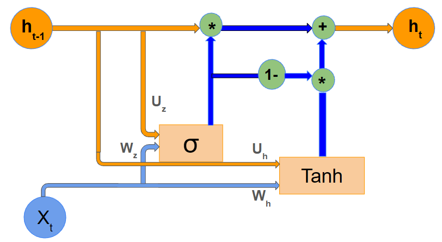
and can be expressed as
where  is the update gate,
 represents the candidate hidden state, and
 is the final hidden state. controls how much of the previous hidden state is preserved versus how much is replaced by the newly proposed state derived from the current input and the past context. is a weighted combination of the previous hidden state and , allowing the network to selectively retain or overwrite information across time steps.
More specifically, is obtained by applying a sigmoid activation function  to an affine combination of the current input
 , the previous hidden state
 that contains the past temporal information, and the bias term
 , where and are first transformed by the learnable weight matrices
 and
 . Similarly,
 is computed by applying a hyperbolic tangent activation
 to an analogous affine transformation of and
 . is computed as a weighted combination of and , where determines how much information is retained from and how much is incorporated from . and
 project into and , respectively, whereas and
 determine how influences and computations. constrains the value of to lie between 0 and 1, while introduces nonlinearity into the modified LiGRU model10. and
 shift the activation values so they are not constrained to pass through zero. Compared to the classical LiGRU cells, this modified version replaced the
 with the and omitted batch normalization to improve fitting.
In this study, a modified LiGRU benchmark and a hybrid quantum-modified LiGRU model, both composed of the GRU cells described above, were developed. The hybrid quantum-modified LiGRU framework was constructed by embedding a quantum circuit, a sequence of transformations applied to qubits, into the update gate and the candidate hidden state of the modified LiGRU model to replace the input-to-hidden transformations  and
 28,29.
Inside the quantum circuit, the inputs to the hybrid quantum-modified LiGRU model were encoded into quantum states, transformed through entangling operations, and then measured into real-valued expectations. More specifically, each input value was converted into a vector consisting of  rotation angles,
where is the number of qubits, and  and
 denote the learnable weight matrix and the bias term, respectively. This transformation mapped the input into a bounded set of angles that can be used to control the quantum gates.
Each angle  in
 was mapped to a parameterized single-qubit rotation gate
which rotates the state of an individual qubit according to the corresponding input angle.
The full encoding operation of was given by the tensor product
Thus, each component of the transformed input is encoded independently onto one of the qubits.
Applying the encoding operator  to the initial state
 yielded the quantum state
where is the basic computational state
In other words, the circuit begins with all qubits in the  state and then applies the input-dependent rotations to obtain the encoded quantum state.
The quantum state was then processed by  entangling layers, with each constructed in the following way:
where  indexes the layer’s position in the circuit,
 is a trainable rotation angle in layer , and
 represents the entire collection of . The CNOT gates were applied in a ring topology, such that each qubit was connected to the next qubit in the circuit. The CNOT gates were chosen because they are commonly used in variational quantum neural networks to create correlations between qubits. These entangling gates allow the information encoded on different qubits to interact30.
The full circuit evolution can be expressed as
where
This expression describes the successive application of all trainable circuit layers to the input-encoded quantum state.
Finally, measurement was performed using the Pauli- operator
and the real-valued expectation was given by quantum feature vector
where  acts on qubit
 . This measurement converts the quantum state into a real-valued quantity that can be passed back into the classical recurrent computation.
The resulting vector  replaces the linear input projections inside the update gate and the candidate hidden state in the following way:
with the computation of the final hidden state left unchanged. An additional output projection linear map  (and, for the candidate gate,
 ) maps the -qubit measurement back to the hidden size
 , so and can stay
 instead of being tied to . In this way, the quantum circuit replaces the direct linear transformation of the current input, while the recurrent dependence on the previous hidden state remains classical. The same
 , generated using the shared encoder and variational circuit parameters, was used for both the update gate and the candidate hidden state transformations. The recurrent transformations and , however, were separately learned for the update gate and the candidate hidden state. For both the modified LiGRU benchmark and the hybrid quantum-modified LiGRU model, the input was a vector of returns at all time steps, and the output was the predicted first difference of the logarithm of the squared daily returns. To confirm the contribution of the quantum component, a series of controlled ablation experiments were conducted in the Monetary Tightening Phase fold by isolating the function of the quantum component. The hybrid quantum-modified LiGRU was compared with a classical feature-map LiGRU that uses a parameter-matched nonlinear transformation, as well as with the variants which have a classical multilayer perceptron, the entangling operations removed, frozen quantum circuits, or separate quantum circuits for the update gate and the candidate hidden state. The same hyperparameter settings were maintained throughout all ablation experiments to ensure a fair comparison. In each experiment, the test RMSE, the test loss, the total number of trainable parameters, wall-clock training time, peak RAM usage were recorded. Training All models were trained to minimize the Mean Squared Error (MSE) loss, defined as
where  denotes the observed target,
 denotes the corresponding model prediction, and
 is the number of observations in the evaluated set. The reported MSE and RMSE values, expressed in the scaled space, are whole-subset metrics computed over all the observations in the corresponding validation or test subsets. To assess whether any observed differences in performance are robust to stochastic variation, all models were trained using 15 random seeds. For each seed, the validation-selected checkpoint was used to select the best model to generate one archived prediction vector under one common aggregation for the held-out test observations and to prevent overfitting. The test RMSE for each seed was calculated as the square root of the corresponding test loss.
The predictive accuracy of each model, evaluated on the validation and the test set, was assessed using RMSE and the loss metric, with the prediction fit graph serving as a supplementary illustration, and then compared across models to evaluate their relative effectiveness. For each fold, the paired differences were calculated as the hybrid quantum-modified LiGRU’s test metric values minus the modified LiGRU’s test metric values and were reported as mean  standard deviation across random seeds. A negative paired difference indicates that the hybrid quantum-modified LiGRU achieved a lower test metric and therefore higher predictive accuracy than the modified LiGRU. The
 confidence intervals (CI) on the paired differences were obtained using a paired time-series-aware block bootstrap. This provides a direct comparison of the predictive performance of the two models. The predictive accuracy was additionally compared using the Diebold-Mariano (DM) test to determine if the forecast errors of two models differ statistically. The null hypothesis of the DM test was that the two models had equal expected predictive accuracy. The Harvey-Leybourne-Newbold small-sample correction was applied to the DM statistic. The statistical significance was assessed using a two-sided significance level of
 . Other than the LiGRU architectures, an Exponential Generalized Autoregressive Heterosdasticity (EGARCH) model and a Linear Regression model were also employed to show whether the hybrid quantum-modified LiGRU framework provided higher accuracy than the baseline methods.
Besides the predictive accuracy, the computational cost of each model in the Monetary Tightening Phase fold was evaluated using the number of trainable parameters, the training time, and the peak RAM usage to compare each model’s resource requirements.
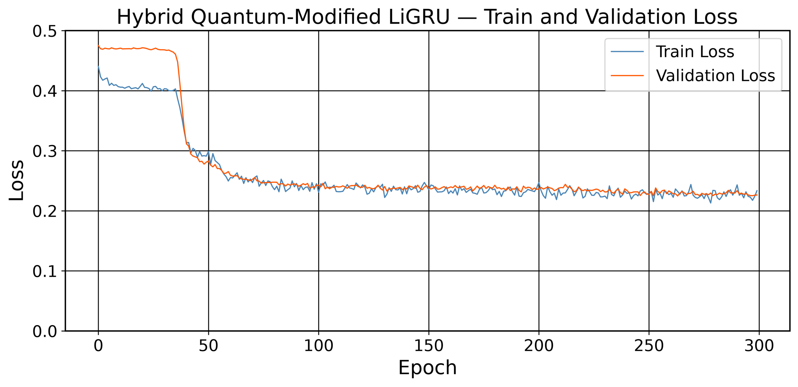
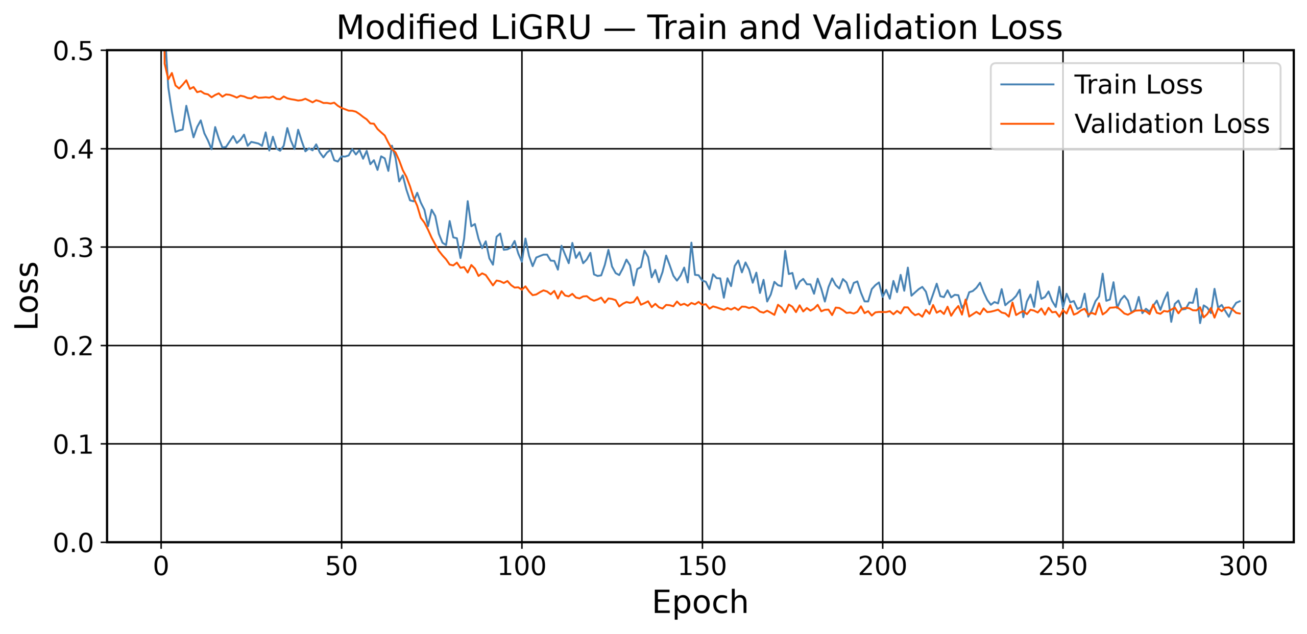
Training was conducted for 300 epochs. Dropout, a technique in which a fraction of neurons is randomly deactivated during training, was applied between cells to reduce the chance of overfitting, where the model performs well on training data but poorly on unseen data31. No additional regularization method, such as L2 weight decay, was applied since no apparent overfitting was observed. A readout function mapped the final hidden state of the last modified LiGRU cell to the output prediction. The Adam optimizer was used for training to improve the convergence stability32. The hyperparameters were selected through grid search separately for each model and fold based on the validation performance. For the hybrid model, the search also included the number of qubits, ranging from 1 to 4, and the number of entangling layers, ranging from 1 to 3. The final hyperparameter configurations are reported in Table 2.
| Fold | Model | Hidden Dim. | Dropout | Learning Rate | Batch Size | Cells | Others |
| Monetary Tightening Phase | Modified LiGRU | 6 | 0.3 | 0.001 | 32 | 2 | N/A |
| Hybrid Quantum -Modified LiGRU | 6 | 0.4 | 0.004 | 64 | 2 | 2 qubits, 1 layer | |
| COVID-19 Shock | Modified LiGRU | 6 | 0.4 | 0.001 | 32 | 2 | N/A |
| Hybrid Quantum -Modified LiGRU | 4 | 0.5 | 0.003 | 64 | 2 | 2 qubits, 1 layer | |
| GFC | Modified LiGRU | 6 | 0.4 | 0.001 | 32 | 2 | N/A |
| Hybrid Quantum -Modified LiGRU | 4 | 0.5 | 0.003 | 64 | 2 | 2 qubits, 1 layer |
In summary, the above experiments and analyses provide a direct assessment of the predictive performance, the statistical robustness, the quantum-specific contributions, the computational cost, the presence of overfitting, and the effect of the data size on the predictive accuracy.
Results
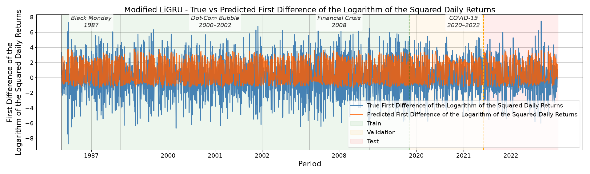
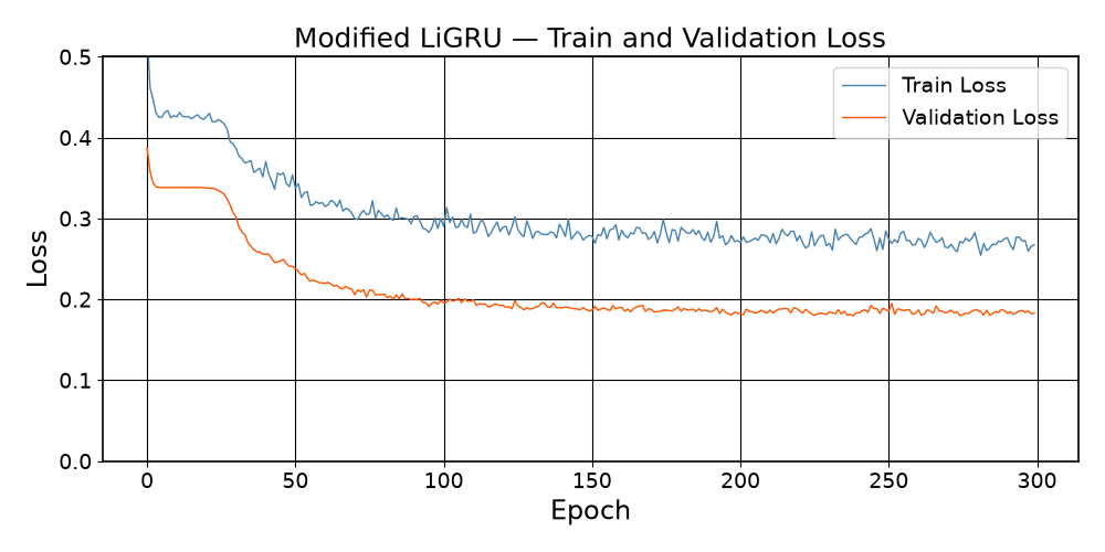
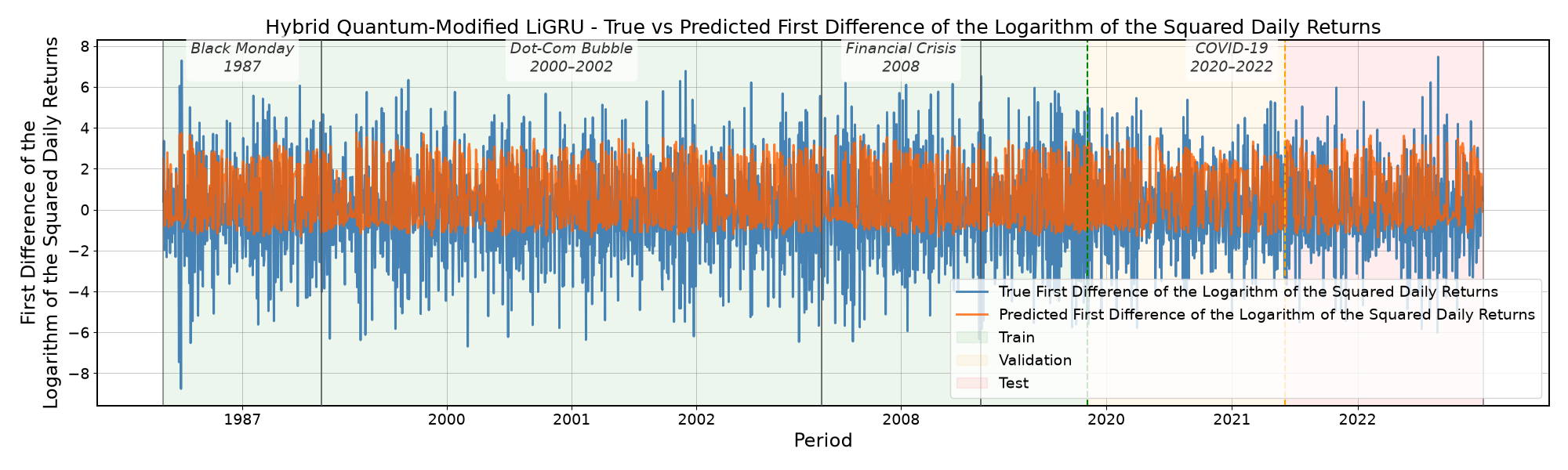
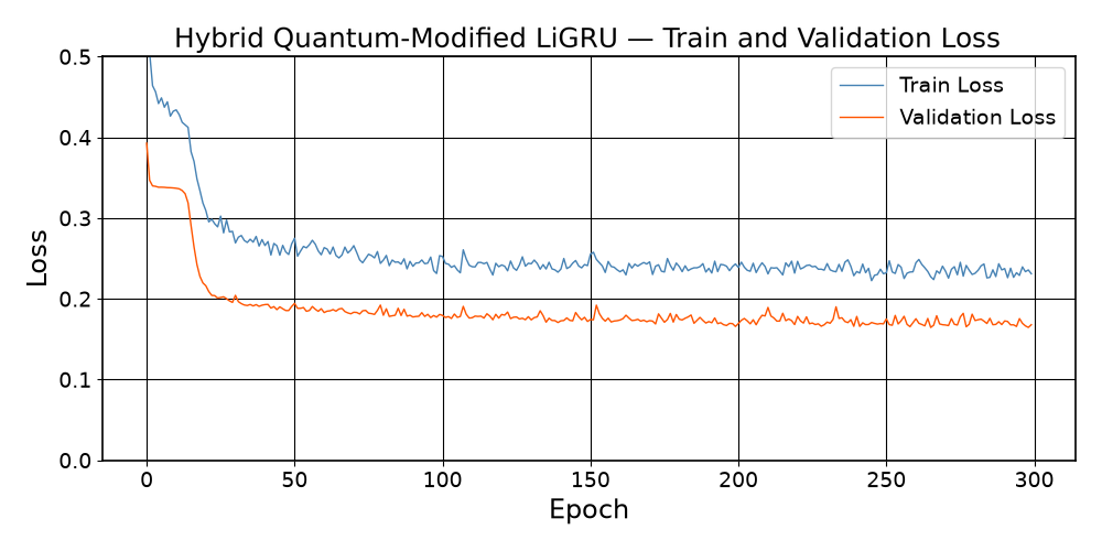
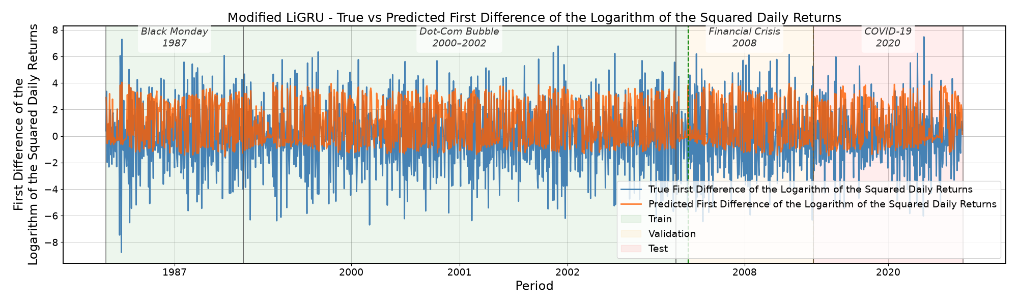
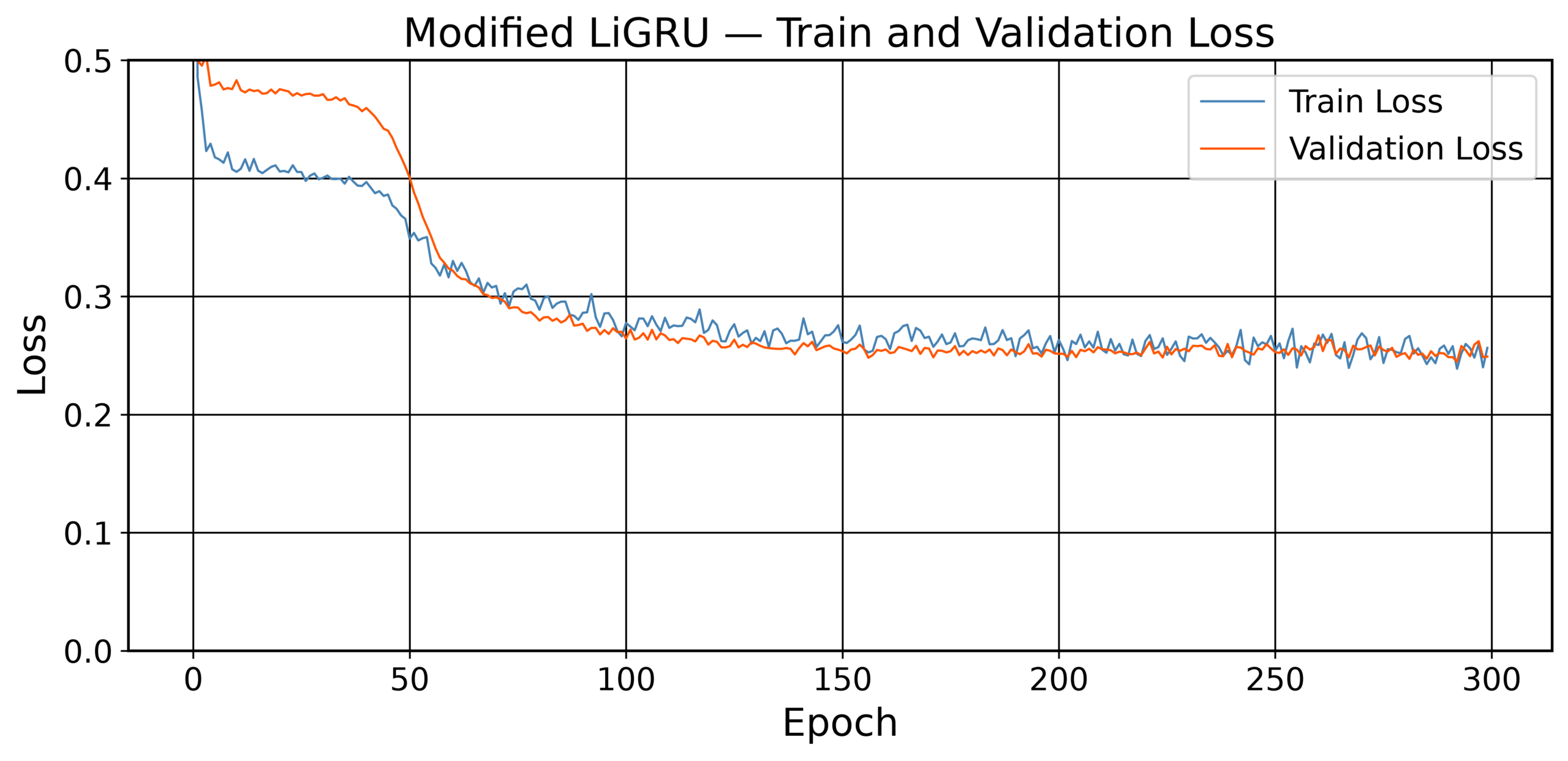
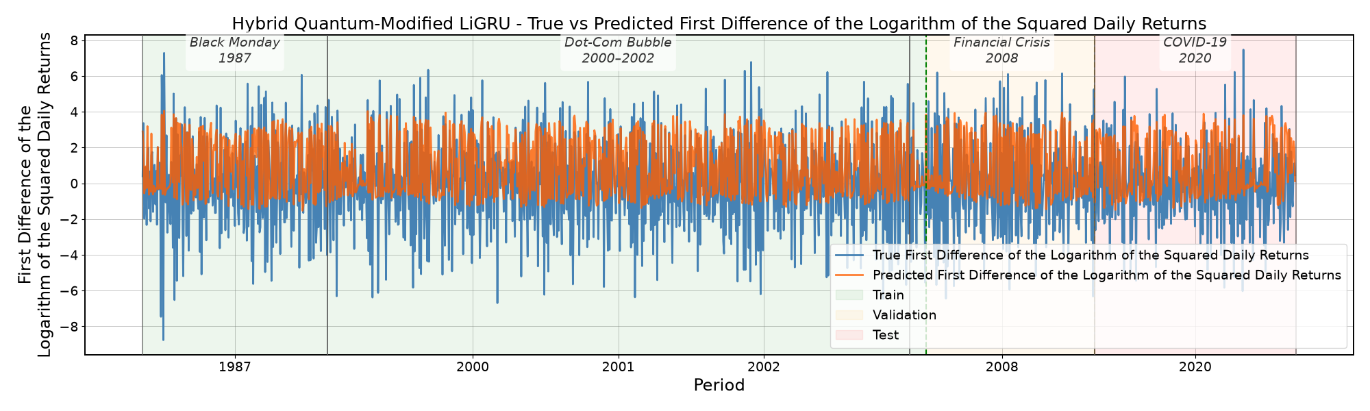
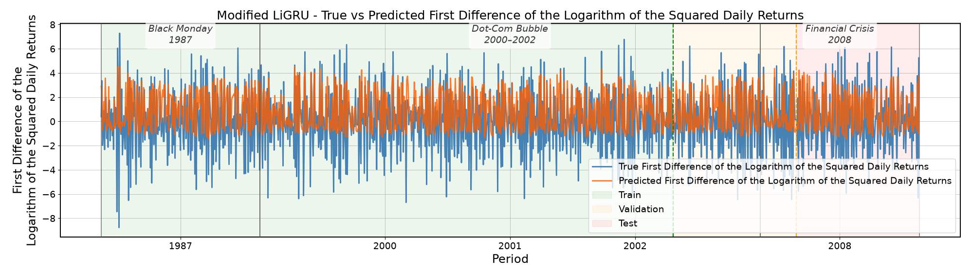
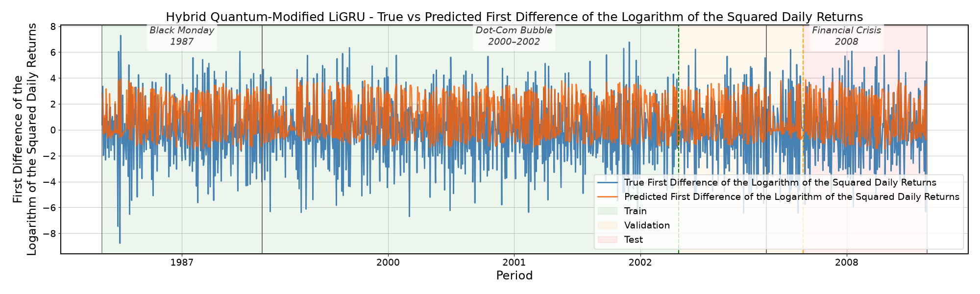
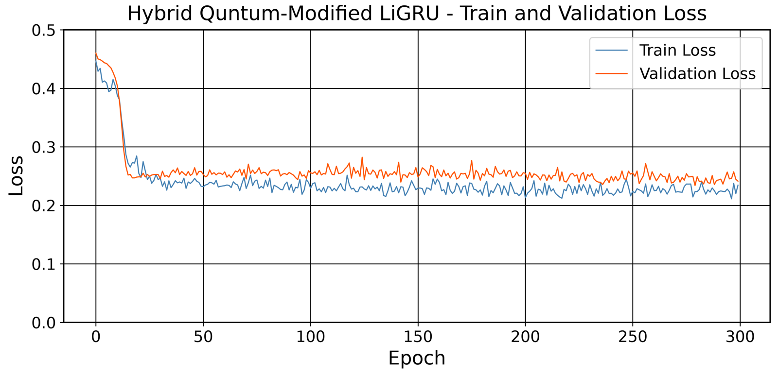
Table 3 summarizes the mean and the standard deviation of the test RMSE and the test loss across the random seeds of the modified LiGRU and the hybrid quantum-modified LiGRU models for each fold, as well as the test RMSE and the test loss of the EGARCH and the Linear Regression models for the Monetary Tightening Phase fold. Table 4 reports the corresponding paired differences between the two models’ test RMSE and test loss values, their 95% bootstrap CIs, and their DM test p-values for each fold. Table 5 reports the results obtained using alternative data splits for the two models for the Monetary Tightening Phase fold. Table 6 compares the trainable parameter count, the training time, and the peak RAM usage of the two models for the Monetary Tightening Phase fold. Table 7 presents the predictive accuracy and the computational cost of the ablation experiments for the Monetary Tightening Phase fold. The prediction fit graph and the train and the validation loss curves for the two models are presented in Figures 2-3, Figures 4-5 and Figures 6-7 for the Monetary Tightening Phase fold, the COVID-19 shock fold and the GFC fold respectively.
| Fold | Model | Test RMSE | Test Loss |
|---|---|---|---|
| Monetary Tightening Phase | Modified LiGRU | 0.443±0.005 | 0.196±0.005 |
| Hybrid Quantum-Modified LiGRU | 0.441±0.009 | 0.195±0.008 | |
| EGARCH | 2.302 | N/A | |
| Linear Regression | 1.833 | 3.351 | |
| COVID-19 Shock | Modified LiGRU | 0.444±0.006 | 0.197±0.005 |
| Hybrid Quantum-Modified LiGRU | 0.451±0.023 | 0.203±0.021 | |
| GFC | Modified LiGRU | 0.474±0.012 | 0.225±0.012 |
| Hybrid Quantum-Modified LiGRU | 0.469±0.040 | 0.221±0.042 |
| Fold | Paired Difference in Test RMSE | Paired Difference in Test Loss | 95% Bootstrap CI Test RMSE | 95% Bootstrap CI Test Loss | DM Test p-value |
|---|---|---|---|---|---|
| Monetary Tightening Phase | -0.002 ± 0.010 | -0.001 ± 0.009 | [-0.006, 0.003] | [-0.007, 0.004] | 0.002 |
| COVID-19 Shock | -0.002±0.008 | -0.001 ± 0.007 | [-0.005, 0.004] | [-0.006, 0.007] | 0.028 |
| GFC | -0.001±0.005 | -0.002 ± 0.003 | [-0.003, 0.002] | [-0.003, 0.005] | 0.754 |
| Split | Model | Test RMSE | Test Loss |
|---|---|---|---|
| 60/20/20 | Modified LiGRU | 0.444±0.007 | 0.196±0.006 |
| Hybrid Quantum-Modified LiGRU | 0.445±0.005 | 0.198±0.005 | |
| 70/15/15 | Modified LiGRU | 0.443±0.005 | 0.196±0.005 |
| Hybrid Quantum-Modified LiGRU | 0.441±0.009 | 0.195±0.008 | |
| 80/10/10 | Modified LiGRU | 0.440±0.003 | 0.193±0.002 |
| Hybrid Quantum-Modified LiGRU | 0.438±0.004 | 0.192±0.002 |
| Model | Number of Trainable Parameters | Training Time (s) | Peak RAM (MB) |
| Modified LiGRU | 451 | 285.714 | 256.390 |
| Hybrid Quantum-Modified LiGRU | 419 | 874.322 | 185.930 |
| Experiments | Test RMSE | Test Loss | Number of Trainable Parameters | Training Time (s) | Peak RAM (MB) |
|---|---|---|---|---|---|
| Hybrid Quantum-Modified LiGRU | 0.441±0.010 | 0.195±0.009 | 419 | 874.322 | 185.930 |
| Quantum Layer Replaced by Classical Layer | 0.475±0.055 | 0.229±0.062 | 419 | 180.000 | 249.060 |
| Entanglement Removed | 0.451±0.022 | 0.204±0.021 | 435 | 173.917 | 245.880 |
| Frozen Circuit | 0.444±0.008 | 0.197±0.007 | 411 | 167.833 | 260.980 |
| Separate Quantum Circuits | 0.441±0.010 | 0.195±0.009 | 419 | 204.583 | 255.730 |
| MLP Replacement | 0.476±0.038 | 0.228±0.039 | 439 | 187.333 | 244.650 |
Discussion
Based on the comparison of the test RMSE, the test loss, the prediction fit graphs, the train and validation loss curves, the number of trainable parameters, the training time, and the peak RAM usage of the hybrid quantum-modified LiGRU and the modified LiGRU architectures, it can be concluded that the hybrid quantum-modified LiGRU model inconsistently provides modest predictive accuracy improvement and incurs substantially higher computational cost than the modified LiGRU model in forecasting the true first difference of the logarithm of the squared daily returns, which partially supports the original hypothesis.
According to Table 3, for the Monetary Tightening Phase fold, the hybrid quantum modified LiGRU achieved a 0.45% lower test RMSE (0.441 vs 0.443) and a 0.51% lower test loss (0.195 vs 0.196) than the modified LiGRU. For the COVID-19 Shock fold, the modified LiGRU modestly outperformed the hybrid quantum-modified LiGRU, achieving a 1.55% lower test RMSE (0.444 vs 0.451) and a 2.96% lower test loss (0.197 vs 0.203). For the GFC fold, the hybrid quantum-modified LiGRU achieved a 1.05% lower test RMSE (0.469 vs 0.474) and a 1.78% lower test loss (0.221 vs 0.225) than the modified LiGRU. The hybrid quantum-modified LiGRU was less stable than the modified LiGRU across all three folds, with a mean test RMSE standard deviation of 0.024 versus 0.008 (213% higher) and a mean test loss standard deviation of 0.024 versus 0.007 (223% higher). Moreover, the results improved as the amount of training data increases: from the GFC fold to the Monetary Tightening Phase fold, the test RMSE of the modified LiGRU fell by 6.54% (0.474 to 0.443) and that of the hybrid quantum-modified LiGRU fell by 5.97% (0.469 to 0.441). This result can be further verified by the different splitting in data illustrated in Table 5. Increasing the training proportion from 60% to 80% lowered the test errors for both models, with test RMSE falling by 0.90% (0.444 to 0.440) for the modified LiGRU and 1.57% (0.445 to 0.438) for the hybrid quantum-modified LiGRU, and test loss falling by 1.53% (0.196 to 0.193) and 3.03% (0.198 to 0.192), respectively, suggesting the hybrid model may benefit more from additional training data. These results also prove that overfitting was not present in either model. According to table 4, The mean paired differences in the test RMSE and the test loss between the hybrid quantum-modified LiGRU and the modified LiGRU were negative across all three folds: -0.002, -0.002, and -0.001 in RMSE, and -0.001, -0.001, and -0.002 in loss for the Monetary Tightening Phase, the COVID-19 Shock, and the GFC folds, respectively. All the negative mean paired differences indicate that the hybrid quantum modified LiGRU model seems to provide slightly higher predictive accuracy. However, the standard deviations indicate substantial variations in the paired differences. Consistent with this, the 95% bootstrap confidence intervals for both the test RMSE and the test loss included zero in all three folds, for example, [-0.006, 0.003] for the RMSE and [-0.007, 0.004] for the loss in the Monetary Tightening Phase fold. These results indicate that the hybrid quantum modified LiGRU provides inconsistent, modest improvements in the predictive accuracy. The DM test gave mixed evidence: the difference was significant in the Monetary Tightening Phase fold (p=0.002) and the COVID-19 Shock fold (p=0.028), but not in the GFC fold (p=0.754). According to Figures 2-7, the true and the predicted first difference of the logarithm of the squared daily returns for both models show a moderately strong positive correlation on the held-out test set and a slightly stronger correlation demonstrated by the hybrid quantum-modified LiGRU, with the Pearson r values for the modified LiGRU being around 0.684 and the hybrid quantum-modified LiGRU being around 0.690. Both LiGRU models outperformed the baselines by a wide margin, with the test RMSE at least 80% lower than the EGARCH (2.302) and at least 75% lower than the linear regression (1.833), and test loss about 94% lower than the linear regression (3.351). Overall, these results suggest that the hybrid quantum-modified LiGRU provides inconsistent, modest improvements in the predictive accuracy.
Based on table 7, the ablation results support that the quantum component contributed to the inconsistent, modest predictive accuracy improvement. The full Hybrid Quantum-Modified LiGRU achieved the best RMSE ( 0.441±0.010 ), outperforming the Classical Layer replacement (0.475 ± 0.055) by  % and the MLP Replacement (0.476 ± 0.038) by 7.4%. Partial-quantum ablations – Entanglement Removed (0.451) and Frozen Circuit (0.444) – landed close to the full model but still trailed it by 2.2% and 0.7% respectively, suggesting entanglement and circuit trainability each added a small incremental gain.
The target used in this study is a volatility-related transformation of daily returns rather than realized volatility or realized variance itself. Specifically, it measures the changes in the logarithm of the squared returns from one day to the next. This transformation focuses the prediction task on short-term changes in return variability, but it does not directly represent the level of realized volatility. Consequently, the results should be interpreted as forecasting changes in this volatility-related target. Future studies could examine alternative volatility measures, including the direct forecast of realized volatility, which should provide a more interpretable measure of market volatility, to determine whether the inconsistent, modest performance observed here persists for other target definitions33. Stronger trend components and non-stationarity are major challenges in direct realized volatility prediction.
The findings may have implications for applications such as options pricing and delta hedging. In particular, variance-forecast errors can contribute to the volatility-mismatch component of delta-hedged P&L, with discrepancies between realized and implied volatility translating into hedging gains or losses34. Thus, volatility forecasting accuracy provides a theoretical basis for evaluating forecasting models in options-hedging applications34. Future research could investigate how metric improvements translate into actual hedging P&L or estimate option mispricing in an example to prove hedging profitability or reduced financial losses35. On the other hand, directly predicting realized volatility may introduce stronger trend and non-stationary components into the target, potentially requiring additional transformations or modeling techniques to account for these properties.
A notable source of error in this research stems from the multifaceted nature of S&P 500 volatility. Market movements can be influenced by numerous interacting factors, including macroeconomic conditions, market sentiment, market microstructure, and investor behavior. Because the present study uses daily returns as the only input feature, the models have access to a limited representation of these underlying factors. Future research could benefit from incorporating richer features beyond stock market daily returns. Moreover, larger datasets containing additional market stress and longer evaluation periods could provide a stronger assessment of whether the inconsistent, modest performance observed in this study generalizes beyond the three folds.
The limitations of classical simulation should be distinguished from the predictive capability of the quantum model itself. The results of future studies that incorporate higher dimensional data could be improved if the quantum circuit was executed on a noisy intermediate scale quantum (NISQ) device, which would enable the use of a greater number of quantum layers and qubits, potentially improving the predictive accuracy36. However, current NISQ devices introduce hardware noise and other implementation errors that may offset potential computational benefits. Future work should empirically evaluate how predictive performance changes with circuit depth, qubit number, entanglement structure, and hardware noise36.
Overall, this study demonstrates the inconsistent, modest predictive advantage for the hybrid quantum-modified LiGRU over the modified LiGRU, with the quantum model providing small improvements in most cases but also incurring higher computational cost. The results therefore suggest that the quantum component is feasible as an alternative feature transformation mechanism within a recurrent forecasting architecture, while its practical predictive benefit remains limited under the small circuit and data conditions examined in this study.
Conclusion
Stock volatility, a key indicator of market behavior, provides valuable insights for both investors and companies. Accurate volatility forecasts can assist investors and firms in making more informed decisions. This study aimed to identify an effective framework for forecasting the true first difference of the logarithm of squared daily returns during the periods of market stress by integrating a quantum circuit with a machine learning approach. Specifically, a hybrid quantum-modified LiGRU model and a modified LiGRU framework were implemented. The hybrid quantum-modified LiGRU was compared to the modified LiGRU model, with predictive accuracy evaluated using the RMSE, the loss metrics, the prediction fit graphs, the paired differences, the bootstrap confidence intervals, and the DM test and computational cost measured using the number of trainable parameters, training time, and peak RAM usage. The results indicate that the hybrid quantum-modified LiGRU achieved inconsistent, modest predictive accuracy improvements and substantially higher computational cost compared to the modified LiGRU model across the evaluated periods of market stress.
The study investigated the potential value of combining the robustness of the modified LiGRU model with the expressive power of the variational quantum circuit for financial prediction tasks. The results give preliminary evidence that quantum-classical RNNs may be useful, but more work is needed before practical deployment. Future research could extend this work by incorporating macroeconomic indicators, market microstructure, and human
behavior variables, as well as testing alternative hybrid neural architectures. Upcoming studies could focus on directly forecasting realized volatility measures as a target variable and executing the quantum circuit on real quantum hardware.
References
- N. Roszyk, R. Ślepaczuk. The hybrid forecast of S&P 500 volatility ensembled from VIX, GARCH and LSTM models. arXiv.org. 2024. [↩]
- M. Otaif. Importance and causes of stock market volatility: Literature review. SSRN Electronic Journal. 2015. [↩]
- W. Bao, Y. Cao, Y. Yang, H. Che, J. Huang, S. Wen. Data-driven stock forecasting models based on neural networks: A review. Information Fusion. Vol. 113, pg. 102616, 2025. [↩] [↩]
- R. Cont. Empirical properties of asset returns: stylized facts and statistical issues. Quantitative Finance. Vol. 1, pg. 223-236, 2001. [↩] [↩]
- T. Phuoc, D. T. Tran, P. H. Tam, T. Q. Nguyen. Applying machine learning algorithms to predict the stock price trend in the stock market – the case of Vietnam. Humanities and Social Sciences Communications. Vol. 11, pg. 393, 2024. [↩] [↩]
- M. R. Bakir, İ. Bakırtaş, E. Ölmez. Statistical techniques vs. machine learning models: A comparative analysis for exchange rate forecasting in Fragile Five countries. Economic Computation and Economic Cybernetics Studies and Research. Vol. 57, pg. 295-312, 2023. [↩] [↩] [↩]
- S. Hochreiter, J. Schmidhuber. Long short-term memory. Neural Computation. Vol. 9, pg. 1735-1780, 1997. [↩] [↩]
- B. Thiesson, D. M. Chickering, D. Heckerman, C. Meek. ARMA time-series modeling with graphical models. arXiv.org. 2012. [↩]
- M. Ravanelli, P. Brakel, M. Omologo, Y. Bengio. Light gated recurrent units for speech recognition. IEEE Transactions on Emerging Topics in Computational Intelligence. Vol. 2, pg. 92-102, 2018. [↩] [↩] [↩]
- H. T. Bao, N. C. Dat, N. D. Anh, H. Thanh-Tung. Learning to Stop Overthinking at Test Time. arXiv.org, 2025. [↩] [↩]
- H. Ye, Y. Zhang, H. Liu, X. Li, J. Chang, H. Zheng. Light Recurrent Unit: Towards an interpretable recurrent neural network for modeling long-range dependency. Electronics. Vol. 13(16), pg. 3204, 2024. [↩] [↩]
- J. V. Tu. Advantages and disadvantages of using artificial neural networks versus logistic regression for predicting medical outcomes. Journal of Clinical Epidemiology. Vol. 49, pg. 1225-1231, 1996. [↩] [↩]
- J. Biamonte, P. Wittek, N. Pancotti, P. Rebentrost, N. Wiebe, S. Lloyd. Quantum machine learning. Nature. Vol. 549(7671), pg. 195-202, 2017. [↩] [↩]
- M. Benedetti, E. Lloyd, S. Sack, M. Fiorentini. Parameterized quantum circuits as machine learning models. Quantum Science and Technology. Vol. 4(4), pg. 043001, 2019. [↩] [↩]
- K. Mitarai, M. Negoro, M. Kitagawa, K. Fujii. Quantum circuit learning. Physical Review A. Vol. 98(3), pg. 032309, 2018. [↩] [↩]
- M. Schuld, N. Killoran. Quantum machine learning in feature Hilbert spaces. Physical Review Letters. Vol. 122(4), pg. 040504, 2019. [↩]
- V. Havlíček, A. D. Córcoles, K. Temme, A. W. Harrow, A. Kandala, J. M. Chow, J. M. Gambetta. Supervised learning with quantum-enhanced feature spaces. Nature. Vol. 567(7747), pg. 209-212, 2019. [↩]
- S. Z. Khan, N. Muzammil, S. Ghafoor, H. Khan, S. M. H. Zaidi, A. J. Aljohani, I. Aziz. Quantum Long Short-Term Memory (QLSTM) vs. classical LSTM in time series forecasting: A comparative study in solar power forecasting. arXiv.org, 2023. [↩]
- Y. Li, Z. Wang, R. Han, S. Shi, J. Li, R. Shang, H. Zheng, G. Zhong, Y. Gu. Quantum recurrent neural networks for sequential learning. Neural Networks. Vol. 166, pg. 148-161, 2023. [↩]
- R. Ahmad, M. Kashif, N. Innan, M. Shafique. Quantum vs. Classical Machine Learning: A Benchmark Study for Financial Prediction. arxiv.org, 2026. [↩]
- K. Kea, D. Kim, C. Huot, T.-K. Kim, Y. Han. A Hybrid Quantum-Classical Model for Stock Price Prediction Using Quantum-Enhanced Long Short-Term Memory. Entropy. Vol. 26, no. 11, pg. 954, 2024. [↩]
- “S&P 500 Historical Data”, Investing.com, 6/20/2026. [↩]
- Z. Dai, X. Zhang, T. Li. Forecasting stock return volatility in data-rich environment: A new powerful predictor. The North American Journal of Economics and Finance. Vol. 64, pg. 101845, 2023. [↩]
- P. Perron, Z. Qu. Long-Memory and Level Shifts in the Volatility of Stock Market Return Indices. Journal of Business & Economic Statistics. Vol. 28, no. 2, pg. 275-290, 2010. [↩]
- J. Li. Predicting Stock Prices of Chinese Liquor Companies with the LSTM Network: A Case Study on Shede Spirits. Highlights in Science, Engineering and Technology. Vol. 57, pg. 180-184, 2023. [↩]
- P. Röchner, H. O. Marques, R. J. G. B. Campello, A. Zimek, F. Rothlauf. Robust statistical scaling of outlier scores: improving the quality of outlier probabilities for outliers (extended version). arXiv.org, 2024. [↩]
- K. Cho, B. van Merriënboer, C. Gulcehre, D. Bahdanau, F. Bougares, H. Schwenk, Y. Bengio. Learning phrase representations using RNN encoder-decoder for statistical machine translation. In Proceedings of the Conference on Empirical Methods in Natural Language Processing (EMNLP), pg. 1724-1734. [↩] [↩]
- V. Bergholm, J. Izaac, M. Schuld, C. Gogolin, S. Ahmed, V. Ajith, M. S. Alam, G. Alonso-Linaje, B. Akash Narayanan, A. Asadi, J. M. Arrazola, U. Azad, S. Banning, C. Blank, T. R. Bromley, B. A. Cordier, J. Ceroni, A. Delgado, O. Di Matteo, A. Dusko, T. Garg, D. Guala, A. Hayes, R. Hill, A. Ijaz, T. Isacsson, D. Ittah, S. Jahangiri, P. Jain, E. Jiang, A. Khandelwal, K. Kottmann, R. A. Lang, C. Lee, T. Loke, A. Lowe, K. McKiernan, J. J. Meyer, J. A. Montañez-Barrera, R. Moyard, Z. Niu, L. J. O’Riordan, S. Oud, A. Panigrahi, C.-Y. Park, D. Polatajko, N. Quesada, C. Roberts, N. Sá, I. Schoch, B. Shi, S. Shu, S. Sim, A. Singh, I. Strandberg, J. Soni, A. Száva, S. Thabet, R. A. Vargas-Hernández, T. Vincent, N. Vitucci, M. Weber, D. Wierichs, R. Wiersema, M. Willmann, V. Wong, S. Zhang, N. Killoran et al. Penny-Lane: automatic differentiation of hybrid quantum-classical computations. arXiv.org, 2018. [↩]
- A. Paszke, S. Gross, F. Massa, A. Lerer, J. Bradbury, G. Chanan, T. Killeen, Z. Lin, N. Gimelshein, L. Antiga, A. Desmaison, A. Köpf, E. Yang, Z. DeVito, M. Raison, A. Tejani, S. Chilamkurthy, B. Steiner, L. Fang, J. Bai, S. Chintala. PyTorch: an imperative style, high-performance deep learning library. Advances in Neural Information Processing Systems. Vol. 32, pg. 8024-8035, 2019. [↩]
- X. Wang, Y. Shi, et al. Theoretical error performance analysis for variational quantum circuit based functional regression. Quantum Information. Vol. 8, 2022. [↩]
- N. Srivastava, G. Hinton, A. Krizhevsky, I. Sutskever, R. Salakhutdinov. Dropout: a simple way to prevent neural networks from overfitting. Journal of Machine Learning Research. Vol. 15(56), pg. 1929-1958, 2014. [↩]
- D. P. Kingma, J. Ba. Adam: a method for stochastic optimization. In 3rd International Conference on Learning Representations (ICLR), 2015. [↩]
- T. G. Andersen, T. Bollerslev, F. X. Diebold. Parametric and Nonparametric Volatility Measurement. NBER Technical Working Paper, No. 0279, 2002. [↩]
- N. El Karoui, M. Jeanblanc-Picqué, S. E. Shreve. Robustness of the Black and Scholes formula. Mathematical Finance. Vol. 8(2), pg. 93-126, 1998. [↩] [↩]
- S.-H. Poon, C. W. J. Granger. Forecasting volatility in financial markets: a review. Journal of Economic Literature. Vol. 41(2), pg. 478-539, 2003. [↩]
- J. Preskill. Quantum computing in the NISQ era and beyond. Quantum. Vol. 2, pg. 79, 2018. [↩] [↩]