

Abstract
Background/Objective. 40% of global energy consumption comes from buildings itself, so being able to estimate how much heating a certain architecture of a building is extremely useful. In our work, we compare three linear regression methods: Ordinary Least Squares (OLS), Ridge, and Lasso, where data is collected from the UCI Energy Efficiency dataset. To zoom in, we look at the accuracy of each method predicting heating load and further determine which architectural features matter the most.
Methods. Each method was written from scratch in NumPy and checked against scikit-learn on an 80/20 train/test split (614 training and 154 test instances, for a total of 768). Every observation of the eight input features contains an exact collinearity, determined through the equation X2=X3+2X4. We evaluated the models on the remaining test set, with 10-fold cross-validation.
Results. The design matrix is rank-deficient (condition number 41015) through the collinearity, and solving the normal equation gives an invalid fit (R2=0.41). To counter this, we use a pseudoinverse; this gives us R2=0.9075, MAE=2.021 kWh/m2, RMSE=2.851 kWh/m2, which matches (to floating-point precision level) scikit-learn. While Ridge Regression (=1.0) reaches R2=0.9081, the paired bootstrap shows that the RMSE advantage does not give a statistical advantage (95% CI [−0.008,0.027] kWh/m2). Our correct implementation of Lasso Regression matches the scikit-learn’s predictions/objective, even though the individual coefficients are related. We organize rankings of features through permutation importance, which places overall height and relative compactness as the most important features.
Conclusions. Ridge and Lasso do not predict heating load better than OLS (regardless of practice/statistical), even though the rank deficiency factor is fixed. Their main benefit is a solution where features are exactly collinear with one another, which OLS fails to do so. Overall height, relative compactness, and glazing area are the most reliable predictors of heating load according to permutation importance.
Keywords: linear regression, Ridge regression, Lasso regression, regularization, building energy efficiency, heating load prediction, multicollinearity, rank deficiency, coordinate descent, permutation importance, cross-validation, bootstrap.
Introduction
Background and Context
40% of global energy consumption1 comes from buildings, so the design and layout of a buildings matters to all ranges of professions (architects, engineers, policymakers, etc.). Having such a model predicting the heating/cooling loads in real life can have many positive implications, such as help stay within building codes, helping energy efficiency runs, etc. Many studies before this one have applied machine-learning to counter this prevalent problem in society, including methods such as basic linear models to gradient-boosted trees, random forests, and deep neural networks. Three issues arise when evaluating recent reviews2,3 : data quality, feature engineering, and the validation of certain models.
Tsanas and Xifara4 created a public dataset that has been widely used in regression manipulation in certain studies. Through the Ecotect simulation tool, they generated 768 building configurations/designs across 12 geometric shapes, including normally extraneous features such as glazing area, glazing distribution, orientation, and more. Each layout has eight main features accounted for: relative compactness ( ), surface area (
 ), wall area (
 ), roof area (
 ), overall height (
 ), orientation (
 ), glazing area (
 ), and glazing area distribution (
 ). The dataset also has two targets, heating load (
 ) and cooling load (
 ), and is within the UCI Machine Learning Repository5. Looking at previous work, most regression studies on this dataset report heating-load
 values from about
 for simple linear baselines to above
 for more complex systems, such as tree ensembles and hybrid models6,7,8. Our linear methods are the more rudimentary end of methods; however, it serves as a more interpretable baseline where everything is mainly derived from scratch. Other work has also noted that vector regression has made a significant impact on fine-tuning a model related to any sort of energy predicting problems9.
Problem Statement and Rationale
A significant problem with this dataset is that one of the features is computed through a linear combination of another two features, defined as “exact collinearity”. This exact collinearity is evident in surface area, where it equals wall area plus twice the roof area, since the buildings accounted in this dataset are closed rectangular shapes. This is the reason why we have a rank-shfit, where the eight-column feature matrix has rank seven, and the intercept column has rank eight instead of nine. A rank-deficient matrix is when the matrix has fewer independent columns (where one doesn’t directly relate); accounting for this, the matrix becomes singular through OLS. However, one predicament that follows this is inversion of the least-squares solution, since explicit inversion does not account for rank deficiency. Instead, we look at the Moore-Penrose pseudoinverse (well-known generalized solution) and QR decomposition with column pivoting.
Significance and Purpose
Estimating heating load early in the design process lets architects compare design choices before committing to construction. Our dataset also shows a problem that is easy to miss; we report how without considering the exact collinearity, different conclusions could potentially be formed about regularization and change how far individual coefficients actually matter.
Objectives
In our work, we calculate OLS to account for the rank deficiency correctly and then compare Ridge10 and Lasso11 against the OLS, allowing us to see the three models’ comparison. Ridge Regression is a popular technique that adds a ℓ2 penalty to the squared-error objective. On the other hand, Lasso Regression is taking the coordinate-descent update so that the threshold matches the objective, which is checked against a trusted solver in different scenarios. Since the raw coefficients for the features weights cannot be determined through exact collinearity, we also report the permutation’s importance, since the uncertainty estimates can be found through every metric.
Scope and Limitations
Our study focuses on heating load (). Cooling load is left for future work () in Section Extension to Cooling Load. For our main comparison we used the regularization parameters ( ) that can be traced from prior work on this dataset (
 ,
 ), and we also report a
 -fold cross-validated to show that this choice does not sort bias in any way. Some limitations of our work include the lack of real building data, where the Ecotect simulations are not from real buildings. Additionally, the linear model might not generate well due to a non-linear relationship existing between features.
Theoretical Framework
Using the linear model  , we find the coefficient vector
 that minimizes any loss over training data12,13. This is done through OLS only, where the residual sum of squares is minimized. Ridge adds a
 penalty, and Lasso adds a
 penalty which punishes the model through minimization. To specify, the penalty stores the solution in a matrix formula and makes the matrix invertible even when the unpenalized matrix is singular. The penalty is not differentiable at zero however, so Lasso uses a popular minimizer technique called coordinate descent, where soft-thresholding updates are used in different conditions14.
Methodology Overview
We derived OLS, Ridge, and Lasso from scratch in NumPy and implemented them on a split of 80/20 (training/test), with features standardized from training-set statistics itself. Every model in Tables 2 and 3 uses the same features, and each from-scratch number in Table 2 has a scikit-learn15 model number as well for comparison. We wrote the from-scratch code to show the math heavy purposes behind regression across different models.
Methods
Research Design
Our work is a comparative, simulation-based data regression study, where the building configurations that Tsanas and Xifara4 generated with Ecotect are available from the UCI Machine Learning Repository5. We use the same 80/20 split for all three model types and for the bootstrap resamples, where the cross-validation (10 fold) is the same across all models as well.
Participants or Sample
The UCI dataset (UCI ID 242, DOI: 10.24432/C51307) has 768 building configurations, having features of 12 geometric shapes generated with Ecotect16. Table 1 lists every variable. Each building has all the same 8 features, along with a heating load target Y1(kWh/m2).
| Code | Feature | Description | Range |
|---|---|---|---|
| X1 | Relative Compactness | Volume-to-surface ratio | –0.98 |
| X2 | Surface Area | Total exterior envelope (m2) | 514–809 |
| X3 | Wall Area | Vertical opaque wall area (m2) | 245–417 |
| X4 | Roof Area | Horizontal footprint (m2) | 110–221 |
| X5 | Overall Height | Building height (m) | 3.5 or 7.0 |
| X6 | Orientation | Cardinal direction (integer code) | 2,3,4,5 |
| X7 | Glazing Area | Window fraction of floor area | 0,0.1,0.25,0.4 |
| X8 | Glazing Area Dist. | Spatial window distribution | 0–5 |
| Y1 | Heating Load | Target: thermal demand (kWh/m2) | 6.01–43.10 |
| Y2 | Cooling Load | Secondary target, Section Extension to Cooling Load | 10.90–48.03 |
Data Collection
All of our data comes directly from the UCI Machine Learning Repository through extraction using the ucimlrepo Python package (fetch_ucirepo(id=242))5. Tsanas and Xifara4 produced the dataset with Ecotect by collecting eight geometric parameters across 12 building types with different layouts and designs (768 configurations).
Variables, Measurements, and Collinearity Diagnostics
The eight input features are described in Table 1. We standardized all of them through z-scores (zero mean and unit variance):
where  and
 are the training-set mean and standard deviation of feature
 . We use these weights to calculate the prediction equation for the test-set as well.
Recall that some of the features rely on other features (exact collinearity), such as the wall area plus twice the roof area:

The raw eight-column in the matrix therefore has rank  and not
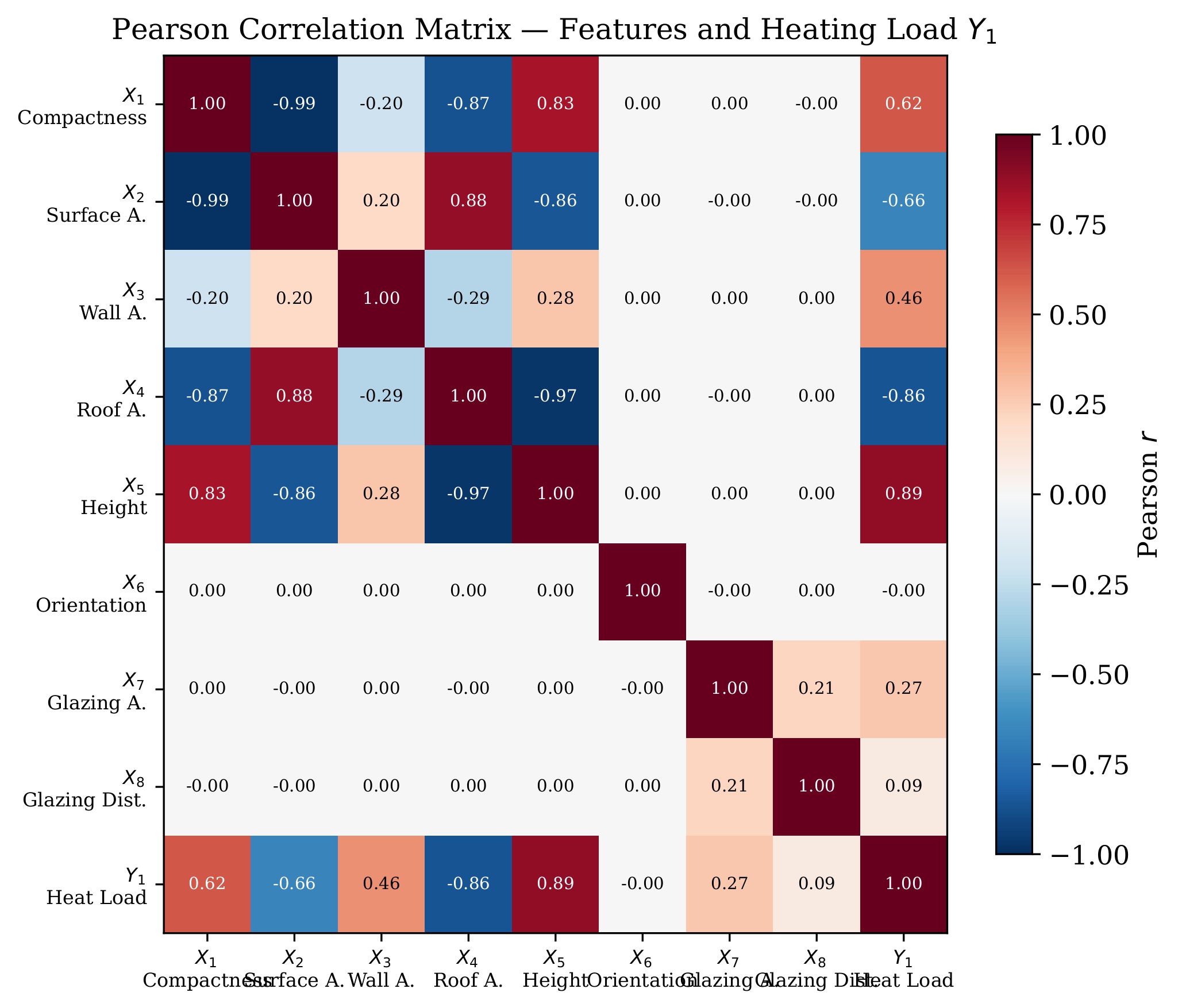
 , and further shifts the columns one back, with the intercept column also shifting from rank 8 to rank 9. Explicit inversion otherwise without the shifting factor would disrupt precision and could potentially produce skewed results due to exact collinearity not being accounted for. , , and all have an infinite variance inflation factor independently, and having larger ones (
 ,
 ) whereas orientation and the glazing features are closer to
 . Through standardization, the Pearson correlation reaches
 proving that the numerical solver used is a valid feature matrix.
Procedure
We split the 768 instances into 80% training ( ) and 20% test (
 ) using a fixed random seed (seed = 42). These metrics are applied for every model (singular-value and variance-inflation diagnostics, which were later compared with scikit-learn’s cross-check). Since a single split gives only a single estimation, we run a 10-fold cross-validation (Section Cross-Validation and Bootstrap Uncertainty), in order to ensure proper evaluation standards. Complete Python code is found in Appendix B.
Data Analysis
Ordinary Least Squares: Rank-Aware Solution of the Normal Equation
Let  be a training set with
 observations and
 features. Augmenting the standardized feature matrix with a column of ones gives:
 .
Definition 1. The OLS main result is through the residual sum of squares,
Theorem 1 (Normal equation, rank-aware form).
If  is invertible, the unique minimizer of
 is

If is singular, the expression is invalid; instead, we look at the Moore–Penrose pseudoinverse,
where  produces a single value decomposition while
 inverts the nonzero single values only.inverts only the nonzero singular values.
Remark 1. Within our study, is a factor that is numerically singular on the UCI dataset (smallest singular value  ). This implementation uses numpy.linalg.lstsq, which applies a singular value decomposition in the end to account for exact collinearity.
Ridge Regression: ℓ2 Regularization
Ridge regression10 takes a different approach through penalization denoted as ℓ2:
Definition 2. Ridge Regression with regularization parameter  is
Theorem 2
(Ridge normal equation). For any  , the unique minimizer of
 is formed through the equation
 where
 does not penalize the intercept.
Proof. For any ,  is defined as positive: the eigenvalues itself are
 for all of
 (since
 ), allowing for invertibility of the augmented matrix even when itself is singular. This minimizer method follows the gradient equation.
Ridge differs to OLS since Ridge implements a penalty (), where said penalty prevents exact collinearity from not inverting, which allows for regularization and high accuracy with precision. As  ,
 approaches the least-squares solution with a smallest coefficient size. We used
 for our main comparison and report the context behind choosing in Section Regularization Path.
Lasso Regression: ℓ1 Regularization and Corrected Coordinate Descent
The Lasso11 replaces the ℓ2 penalty with an ℓ1 norm:
Definition 3. The Lasso objective with regularization parameter is
Because  is not differentiable at
 , we implement a gradient technique called coordinate descent17, which updates one coefficient at a time. For coordinate with all other coordinates fixed, the ordinary-least-squares partial fit is recalled as
 , and the squares of the differences is denoted as
 . This gives us our partial residual predictor called
 .
Definition 4 (Soft-thresholding). For  and
 :

Proposition 1. The coordinate update for Lasso Regression is 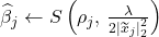 for
 , and
 for the intercept.
Since , , and are exactly collinear, the fitted values of the Lasso solution to  are unique but the coefficients are not. We used
 for our main comparison, in which it preserves the three dependent columns and their linear contributions. This is compared with scikit-learn’s coordinate descent method itself.
Evaluation Metrics, Cross-Validation, and Bootstrap Protocol
Three metrics are computed from scratch on the test set (ntest=154):
A 80/20 split gives only singular estimates of these metrics, so we use two additional approaches to measure the validity of the regression models. First, 10-fold cross-validation18 splits the data into ten parts and is refitted into every model on nine of them and finally evaluated on the tenth fold. This repeats with reportage of mean and standard deviation. Second, a bootstrap19 with B=5,000 resamples of the test set is also conducted, where each resample is replaced from the test set. This gives 95% confidence rates for RMSE. Additionally, the implementation of a paired bootstrap on the same resamples gives a RMSE difference between OLS and Ridge, letting us test whether one model beats the other consistently.
Permutation Importance
Exact collinearity has an issue of not having unique coefficients for each regression model, so we implement and report permutation importance as well. For each feature and fitted model  , we shuffle the values per feature across the test observations, re-evaluate the model, and record how much RMSE increases overtime. We iterate this 100 times for each feature and report the mean and standard deviation, further measuring any increase as well. If shuffling a feature leaves RMSE unchanged, we can infer that the model does not rely on that certain feature as much, so the weight must be lower than other more important features. An important fact to note however is that permutation importance could be biased toward correlated predictors20, which we acknowledge during evaluation.
Ethical Considerations
All of the data is public and comes from the UCI Machine Learning Repository5, and all data is simulated building layout types instead of real-world data collected.
Results
Predictive Performance and Correction of the Numerical Error
When we use the OLS normal equation (Theorem 1) by explicit inversion (without accounting for exact collinearity), we get R2=0.408, MAE=6.138 kWh/m2, and RMSE=7.214 kWh/m2 generated from the test set without errors. With the pseudoinverse method (accounting for exact collinearity), we generate R2=0.9075, MAE=2.021 kWh/m2, RMSE=2.851 kWh/m2, with an intercept of 22.656. Further looking into the statistics, the mean of Y1 evaluates to five decimal places, further matching theory. This corrected solution matches scikit-learn’s LinearRegression to a tolerance of 10−10 in every reported weight, so Table 2 reports a single OLS row instead of two disagreeing ones.
| Model | λ | R2 | MAE (kWh/m2) | RMSE (kWh/m2) | scikit-learn agreement |
| OLS, explicit inversion (uncorrected) | — | 0.408 | 6.138 | 7.214 | n/a |
| OLS, pseudoinverse (corrected) | — | 0.9075 | 2.021 | 2.851 | to 10−10 |
| Ridge | 1.0 | 0.9081 | 2.009 | 2.841 | to 10−10 |
| Lasso, corrected threshold | 0.1 | 0.9075 | 2.021 | 2.851 | pred. to 710−4 |
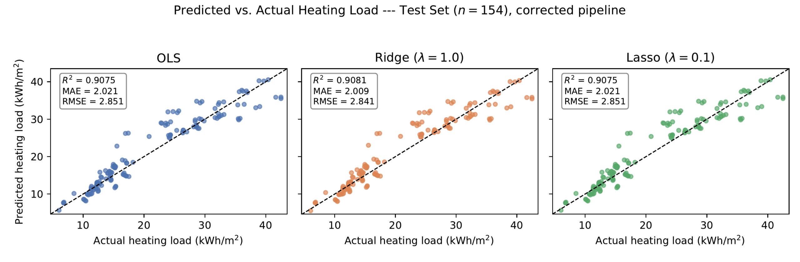
 ). All three models track
 ; as shown in the plotted diagram, the larger error at higher values is proved through the same nonlinear structure briefly mentioned in Section Residual Diagnostics.
Ridge’s performance has a slight improvement over OLS ( lower by
 , higher by
 ). A paired bootstrap over
 produces a 95% confidence interval for
 , the interval being
 . Ridge has the lower resampled RMSE (
 ) of the models, but this does not have much significance in the long run. Repeated -fold cross-validation shows the same pattern (larger dataset), so the RSME will balance out. On this dataset, both methods have the same accuracy as OLS in accuracy and have a more stabler approach when considering exact collinearity.
Validation of the Corrected Lasso Implementation
We checked our coordinate-descent Lasso gainst scikit-learn’s Lasso, rescaling its penalty ( ) and not penalizing the intercept. On the training set, both the computed and the derived methods agree on all metrics within
 and on the value itself (within
 :5,315.78 vs. 5,315.58). On the other hand, they do not agree on individual coefficients: the derived version generates
 to and
 to , , while scikit-learn generates
 to and
 to . Since , , and are exactly collinear, the Lasso predictions are unique, but the coefficients are not, since Lasso Regression does not account for exact collinearity.
Coefficient Analysis and Its Limits
Table 3 shows the coefficients that were run through standardization. Because of the exact collinearity, the coefficients in one solution are not the only solution that fits; coefficients can be changed and still have consistent results, allowing for multiple solutions. Overall height has the largest positive coefficient in all three models. This can be interpreted in a real-world context, where taller buildings expose more volume and therefore demand more heating. Glazing area is positive as well, but not as much as overall height. Orientation has a near-zero coefficient in every model and does not depend on how the collinear features are decomposed.
| Feature | OLS | Ridge (λ=1.0) | Lasso ( λ=0.1) |
|---|---|---|---|
| X1 : Relative Compactness | −7.312 | −5.998 | −7.299 |
| X2 : Surface Area* | −4.043 | −3.162 | −7.057 |
| X3 : Wall Area* | 0.637 | 0.860 | 2.124 |
| X4 : Roof Area* | −4.269 | −3.513 | −1.176 |
| X5 : Overall Height | 7.289 | 7.620 | 7.294 |
| X6 : Orientation | −0.086 | −0.084 | −0.086 |
| X7 : Glazing Area | 2.593 | 2.586 | 2.593 |
| X8 : Glazing Area Dist. | 0.305 | 0.306 | 0.305 |
 (training-set mean of ) for OLS and Ridge. Coefficients for
 are not unique (exact collinearity); one valid solution is shown.
 Not uniquely determined: are exactly collinear, so these three values do not depend on predictions.
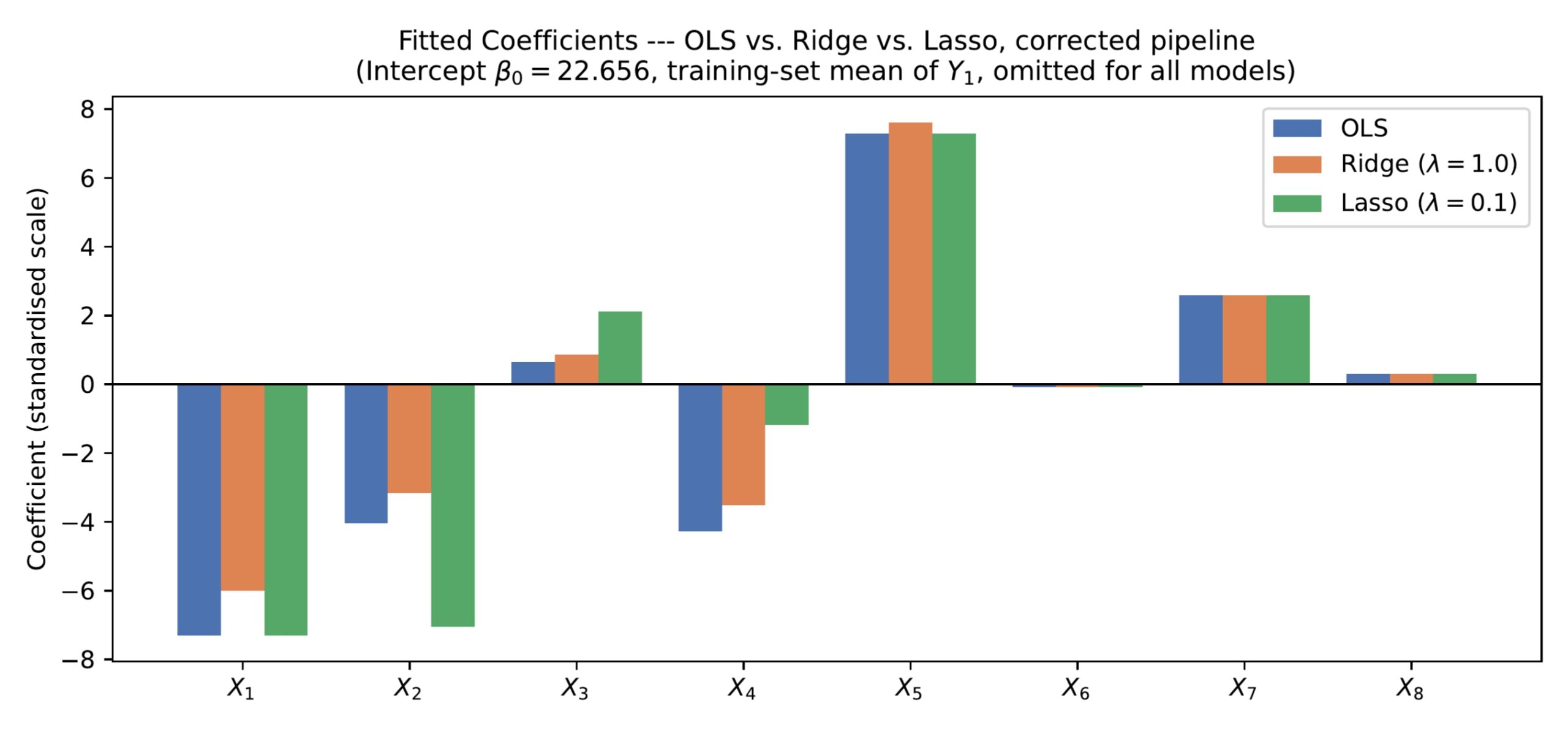 , , , and the near-zero , but disagree on how they split weight among the exactly collinear , , (not accounted for)
Permutation Importance
Figure 4 shows the mean increase in test RMSE, when we shuffle each feature in the test set and re-evaluate the Ridge model without refitting. Overall height (X5, RMSE increase 7.980.41 kWh/m2) and relative compactness (X1, 6.220.37) have more weightage than any other feature. Moderate weights include roof area, surface area, and glazing area, and wall area and glazing distribution contribute very little, and orientation has almost zero effect (−0.0050.007).
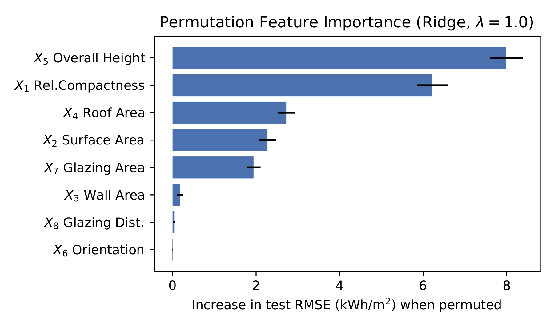 ), test set has
 iterations per feature. Error bars are also included.
Regularization Path
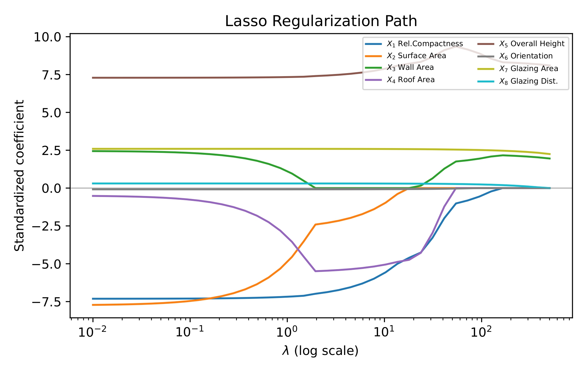
Figure 5 sweeps and plots each standardized coefficient against , fitted on a log scale. Test performance is flat for the most part, with ≲6 and RMSE barely changing (only in third decimal place)/ All eight coefficients stay nonzero, so the regression never breaks. Coefficients first reach exactly zero between 6 and 24, where wall area and glazing distribution are the first to becom exactly 0. RMSE on the test set is lowest near 24 (RMSE=2.840 kWh/m2) and inflates at ≳130, where the penalty starts removing important weights that are needed to fit the regression. The value =0.1 that we used for our main comparison therefore is valid, as it does not make any coefficients exactly zero or removes important weights.
Cross-Validation and Bootstrap Uncertainty
Repeated 10-fold cross-validation over all 768 samples gives R2=0.91410.0130, MAE=2.0830.241 kWh/m2, RMSE=2.9300.257 kWh/m2 for OLS and R2=0.91400.0128, MAE=2.0840.239 kWh/m2, RMSE=2.9310.259 kWh/m2 for Ridge (=1.0, one in ten folds). The two models’ metrics do not differ by much. There are no seen improvements in OLS and Ridge, when organized by ordinary sampling variability. The cross-validated R2 is also slightly higher than single-split (Table 2: 0.914 vs. 0.908), which shows the limitations of using a single-split model.
Residual Diagnostics
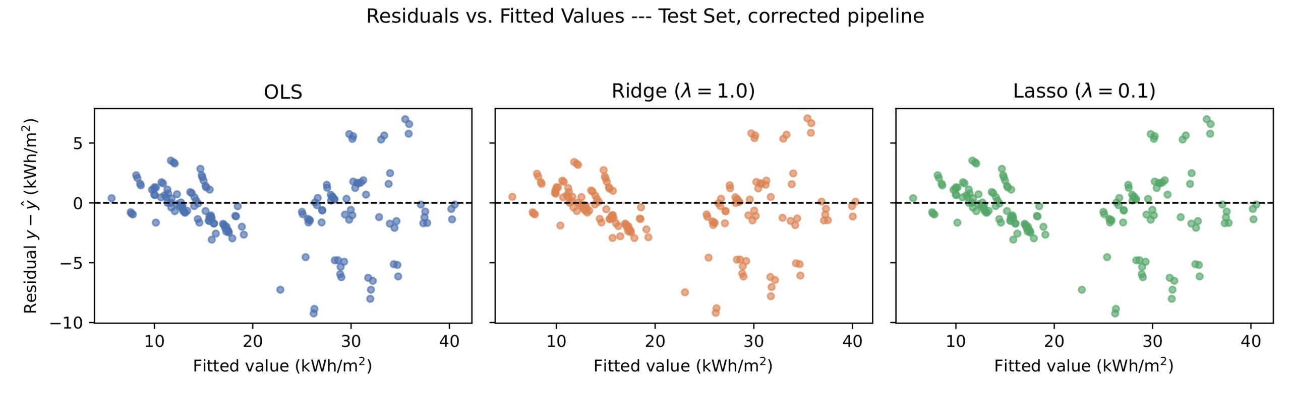
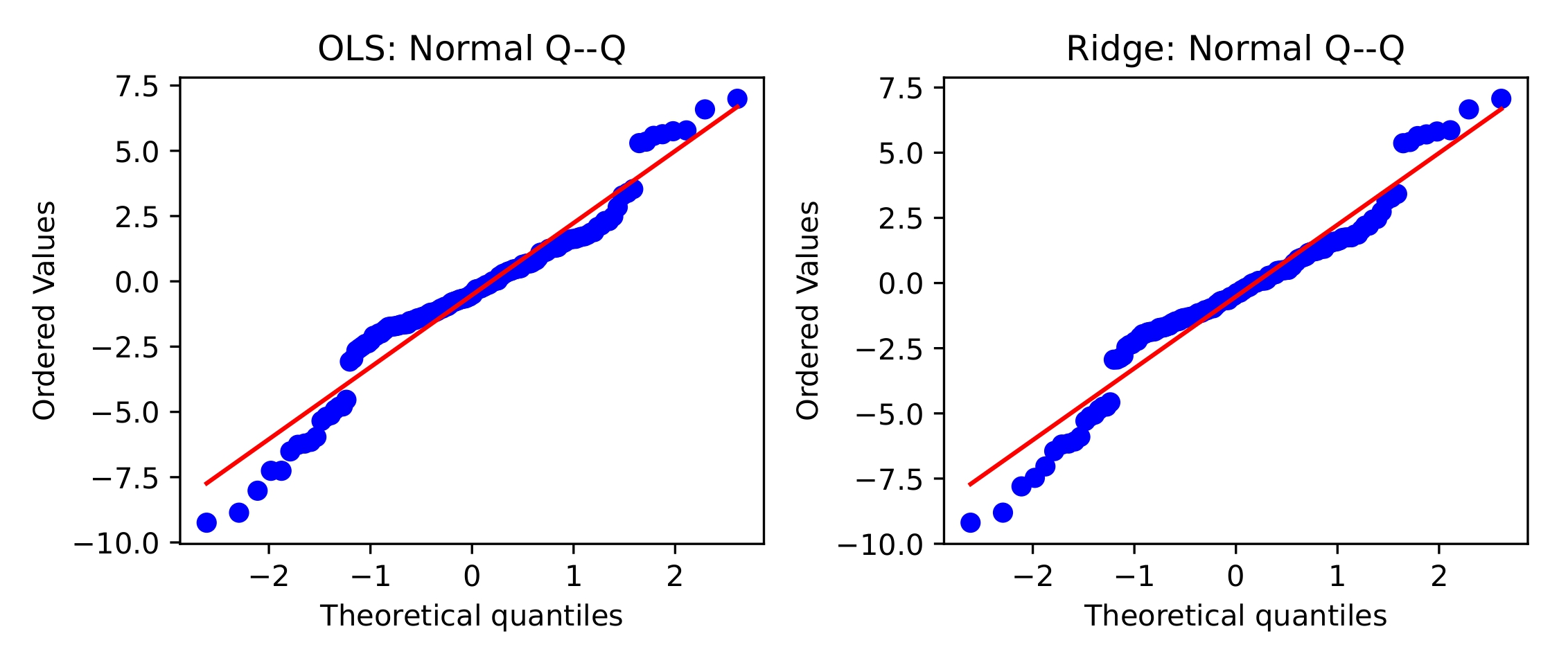
Figure 6 plots the residuals against the values for the three models. All three models have the same fan-shaped spread, with large positive residuals seen more at lower values. Lasso’s residuals and Ridge’s residuals are almost identical, as well as the RMSE in both models (a difference of 0.0004 kWh/m2). Figure 7 shows quantile-quantile plots for OLS and Ridge, and both deviate from the reference line in the upper section. To test normallity, we conduct a Shapiro–Wilk test21, which rejects normality in both scenarios (OLS p=1.110−5; Ridge p=1.310−5). These diagnostics suggest that the error is not present in normality; it comes from nonlinear structure that our models cannot capture, so changing will not change the outcome.
Baseline Comparisons
To show  in context of models, we ran two baselines on the same test split. A constant model that always predicts the test-set mean gives
 (not the training-set mean, so the value will be lower) and
 . As a comparison with OLS using one feature (overall height (): the top feature by permutation importance), we get
 and
 . Therefore, the other seven features reduce RMSE by a further
 , from
 to
 .
Orientation Encoding
Orientation () is numerated as integers  as the four cardinal directions that the building could potentially face in the Ecotect simulation that the data was collected from. Since it is a categorical variable and we cannot assign a numerical value, the coefficient could be changed due to using the above integers as cardinal directions. To test this, we replaced the integer column with a one-hot encoding column (three indicator columns, with one level dropped) and reran OLS using non-numerical values for the cardinal directions. moved from
 to
 and RMSE from
 to
 , which tells us that orientation carries almost no information about heating load under encoding as well.
Extension to Cooling Load
As a quick check on how the statistics change, we use the same pipeline for cooling load () on the same 80/20 split. OLS achieves  ,
 ,
 , and Ridge () achieves
 ,
 ,
 , so accuracy is lower than heating load. The leading coefficients follow the same sign pattern: strongly negative for compactness-related (volume) features and very positive for height and glazing area. A full multi-output treatment, with its own permutation importance and regularization path for , is not covered in this study and is left for future work.
Discussion
Restatement of Key Findings
Once we handle the exact collinearity constraint by using a pseudoinverse instead of explicit inversion, there is little to no accuracy advantage between Ridge, Lasso, and OLS. The RMSE gap between corrected OLS and Ridge is 0.010 kWh/m2 and holds no advantage from zero under both a paired bootstrap in addition to a 10-fold cross-validation. Regularization provides a stable solution while having the constraint of rank deficiency, allowing Ridge to be inverted in any collinearity and OLS to be computed the same way with treating rank deficiency. Permutation importance places overall height and relative compactness as more weighed than the other features; glazing area contributes a moderate amount, and orientation adds little to no support under either integer coding or one-hot encoding.
Implications and Significance
Overall, height and compactness have the largest effect on predicted heating demand by a large margin, and both the coefficients and the permutation importance lead to this conclusion. Glazing area matters have moderate effects, so the glazing specification (for example double glazing or low-emissivity coatings) is a reasonable feature that can determine the possible heating demand. Orientation shows very little to no effect on heating load under encoding. Additionally, wall, surface, and roof area are exactly collinear, so a linear coefficient table cannot be used and can further bias the output if used in conjunction.
Connection to Objectives
We met all four of our goals. Our pseudoinverse-based OLS matches scikit-learn’s LinearRegression on the identical split to floating-point precision, and Ridge makes the matrix invertible despite the exact rank deficiency. Our corrected Lasso solver agrees with scikit-learn on fitted values and objective value, which are the quantities that are uniquely determined here, since individual coefficients are provably not unique. Cross-validation and bootstrap intervals give an explicit measure of uncertainty for our reported metrics, and permutation importance ranks features without relying on the coefficients.
Recommendations
We see four ways to extend this work. Including the cooling load would be a first piority, with a shared regularization path between cooling and heating, as well as separate permutation importance for each. Nonlinear models are the next thing to try, since our residual graph indicates a nonlinear fit that is superior to an OLS, Ridge, or Lasso model. Gradient-boosted trees22 and random forests23 have been used in past studies, where R2 above 0.99 on this dataset in other work3,8. An elastic net combines ℓ1 and ℓ2 penalties24, which would let a single model cover the range from Ridge to Lasso.
Limitations
Our dataset consists of simulations and not measurements of real buildings, which may limit our results in the real world. As we mentioned before, the nonlinear model features cannot be captured in a linear model, so the accuracy metric cannot be captured with a linear regression. Additionally, the Lasso coefficient table should not be the main metric of evalution for X2, X3, X4, for the reasons given in Section Validation of the Corrected Lasso Implementation (not considering exact collinearity), and for those features we instead use a different method of approach given in Section Validation of the Corrected Lasso Implementation.
Conclusions
In this paper, we first have three features that are exactly linearly dependent. This makes the OLS normal equation invalid with explicit inversion, and we introduce a psuedoinverse solution. This matches scikit-learn to extreme precision (R2=0.9075, RMSE=2.851 kWh/m2). With this correction, Ridge and Lasso have no accuracy advantage over OLS under either a paired bootstrap or 10-fold cross-validation. In terms of stability, Ridge is more stable due to having an always unique solution despite the collinearity. On the other hand, Lasso also matches scikit-learn on objective value, confirming individual coefficients among the three exact collinear features are not unique. Through permutation importance, overall height and relative compactness are the most reliable predictors of heating load, followed by glazing area, and orientation adds little to no information under either an integer or one-hot encoding. The remaining error is that the pattern is in a nonlinear structure, which a linear model cannot capture.
Acknowledgments
Special thanks to PhD Candidate William Legg for mentoring this research, as well as teaching the main fundamentals behind each model of regression.
Appendix A. Notation Index
| Symbol | Meaning |
|---|---|
 | Number of training observations (614) |
 | Number of features (8) |
 | Standardized feature matrix |
| Augmented design matrix (intercept prepended) |
 | Heating load target vector |
 | Coefficient vector (intercept + p slopes) |
 | OLS coefficient estimate (pseudoinverse solution) |
| Ridge coefficient estimate |
 | Lasso coefficient estimate |
| Regularization hyperparameter |
 | Moore–Penrose pseudoinverse of X |
 | Modified identity: diag(0,1,,1); excludes intercept |
 | Soft-thresholding operator (Definition 4) |
 | Unconstrained coordinate-wise minimizer for Lasso update |
 | Variance inflation factor for feature j |
| Coefficient of determination (fraction of variance explained) |
| MAE | Mean Absolute Error (kWh/m2) |
| RMSE | Root Mean Squared Error (kWh/m2) |
Appendix B. Coding Implementation
All estimators are implemented in Python 3 using NumPy; scikit-learn is used as a cross-validation reference.
B.1 Data Access, Split, and Standardization (unchanged)
from ucimlrepo import fetch_ucirepo
import numpy as np
energy_efficiency = fetch_ucirepo(id=242)
X = energy_efficiency.data.features.values # shape (768, 8)
y = energy_efficiency.data.targets[‘Y1’].values
np.random.seed(42)
indices = np.random.permutation(768)
split = int(0.8 * 768)
train_idx, test_idx = indices[:split], indices[split:]
X_train, X_test = X[train_idx], X[test_idx]
y_train, y_test = y[train_idx], y[test_idx]
X_mean, X_std = X_train.mean(axis=0), X_train.std(axis=0)
X_train_scaled = (X_train – X_mean) / X_std
X_test_scaled = (X_test – X_mean) / X_std
B.2 OLS: Corrected, Rank-Aware Solution
X_b = np.c_[np.ones(X_train_scaled.shape[0]), X_train_scaled]
# Earlier (invalid on this rank-deficient matrix):
# beta = np.linalg.inv(X_b.T @ X_b) @ X_b.T @ y_train
# Corrected: rank-aware least-squares solve.
beta, residuals, rank, sv = np.linalg.lstsq(X_b, y_train, rcond=None)
print(“design matrix rank:”, rank, “of”, X_b.shape[1], “columns”)
print(“singular values:”, sv)
intercept, coefficients = beta[0], beta[1:]
B.3 Ridge Regression (unchanged apart from reuse of the shared split)
lambda_ = 1.0
I = np.eye(X_b.shape[1]); I[0, 0] = 0
beta_ridge = np.linalg.solve(X_b.T @ X_b + lambda_ * I, X_b.T @ y_train)
B.4 Lasso via Corrected Coordinate Descent
def soft_threshold(rho, tau):
if rho > tau: return rho – tau
elif rho < -tau: return rho + tau
else: return 0.0
def lasso_coordinate_descent(X, y, lambda_=1.0, max_iter=20000, tol=1e-9):
X_b = np.c_[np.ones(X.shape[0]), X]
n, p = X_b.shape
beta = np.zeros(p)
col_sqnorm = np.sum(X_b**2, axis=0)
for iteration in range(max_iter):
beta_old = beta.copy()
for j in range(p):
residual = y – X_b @ beta + X_b[:, j] * beta[j]
rho = (X_b[:, j] @ residual) / col_sqnorm[j] # normalized rho_j
if j == 0:
beta[j] = rho # unpenalized intercept
else:
tau = lambda_ / (2.0 * col_sqnorm[j]) # matching threshold
beta[j] = soft_threshold(rho, tau)
if np.max(np.abs(beta – beta_old)) < tol:
break
return beta
beta_lasso = lasso_coordinate_descent(X_train_scaled, y_train, lambda_=0.1)
B.5 Cross-Validation, Bootstrap, and Permutation Importance
# 10-fold cross-validation (mean +/- std across folds), reusing fit_eval() as in B.2-B.3
rng = np.random.RandomState(42)
folds = np.array_split(rng.permutation(len(y)), 10)
scores = []
for i in range(10):
te = folds[i]
tr = np.concatenate([folds[j] for j in range(10) if j != i])
scores.append(fit_eval_ols(X[tr], y[tr], X[te], y[te])) # returns (R2, MAE, RMSE)
scores = np.array(scores)
print(scores.mean(axis=0), scores.std(axis=0))
# Paired bootstrap: RMSE(OLS) – RMSE(Ridge) on the fixed test set
rng = np.random.RandomState(1)
pred_ols, pred_ridge = X_b_test @ beta, X_b_test @ beta_ridge
diffs = []
for _ in range(5000):
idx = rng.randint(0, len(y_test), len(y_test))
rmse_o = np.sqrt(np.mean((y_test[idx] – pred_ols[idx])**2))
rmse_r = np.sqrt(np.mean((y_test[idx] – pred_ridge[idx])**2))
diffs.append(rmse_o – rmse_r)
print(“95% CI:”, np.percentile(diffs, [2.5, 97.5]))
# Permutation importance for feature j, model beta, on the test set
def permutation_importance(beta, X_test_scaled, y_test, j, n_repeats=100, seed=0):
rng = np.random.RandomState(seed)
base_rmse = rmse_of(beta, X_test_scaled, y_test)
increases = []
for _ in range(n_repeats):
Xp = X_test_scaled.copy()
Xp[:, j] = Xp[rng.permutation(len(Xp)), j]
increases.append(rmse_of(beta, Xp, y_test) – base_rmse)
return np.mean(increases), np.std(increases)
B.6 Evaluation Metrics (unchanged)
X_test_b = np.c_[np.ones(X_test_scaled.shape[0]), X_test_scaled]
y_pred = X_test_b @ beta
ss_res = np.sum((y_test – y_pred)**2)
ss_tot = np.sum((y_test – y_test.mean())**2)
r2 = 1 – ss_res / ss_tot
mae = np.mean(np.abs(y_test – y_pred))
rmse = np.sqrt(np.mean((y_test – y_pred)**2))
Appendix C. Derivation of the Corrected Soft-Thresholding Operator
This appendix corrects the orginal derivation, which stated the coordinate as  and had a threshold of
 , which is not derivable. Using the equation revolved around the paper,
 , the coordinate-wise subproblem for
 , after completing the square around , is

The subdifferential of is

where  for
 and
 . The overall minimizer satisfies
 . For
 ,
 , valid when
 ; symmetrically for
 ; and
 is required when
 . Combining all three cases, which is Definition 4 evaluated at threshold
 .
References
- International Energy Agency. Buildings – tracking clean energy progress. IEA, Paris, 2023. https://www.iea.org/energy-system/buildings. [↩]
- L. Zhang, J. Wen, Y. Li, J. Chen, Y. Ye, Y. Fu, W. Livingood. A review of machine learning in building load prediction. Applied Energy. Vol. 285, 116452, 2021, https://doi.org/10.1016/j.apenergy.2021.116452. [↩]
- S. Seyedzadeh, F. P. Rahimian, I. Glesk, M. Roper. Machine learning for estimation of building energy consumption and performance: a review. Visualization in Engineering. Vol. 6, 5, 2018, https://doi.org/10.1186/s40327-018-0064-7. [↩] [↩]
- A. Tsanas, A. Xifara. Accurate quantitative estimation of energy performance of residential buildings using statistical machine learning tools. Energy and Buildings. Vol. 49, pg. 560–567, 2012, https://doi.org/10.1016/j.enbuild.2012.03.003. [↩] [↩] [↩]
- D. Dua, C. Graff. UCI machine learning repository: energy efficiency dataset (ID 242). https://archive.ics.uci.edu/dataset/242/energy+efficiency, 2024. DOI: 10.24432/C51307. [↩] [↩] [↩] [↩]
- M. Ahmadi. Building energy efficiency: using machine learning algorithms to accurately predict heating load. Asian Journal of Civil Engineering. Vol. 25, pg. 3129–3139, 2024, https://doi.org/10.1007/s42107-023-00967-w. [↩]
- M. W. Ahmad, M. Mourshed, Y. Rezgui. Trees vs neurons: comparison between random forest and ANN for high-resolution prediction of building energy consumption. Energy and Buildings. Vol. 147, pg. 77–89, 2017, https://doi.org/10.1016/j.enbuild.2017.04.038. [↩]
- M. S. Farooq et al. Building heating and cooling load prediction using ensemble machine learning model. Sensors. Vol. 22, no. 24, 9694, 2022, https://doi.org/10.3390/s22249694. [↩] [↩]
- K. Kavaklioglu. Modeling and prediction of Turkey’s electricity consumption using support vector regression. Applied Energy. Vol. 88, pg. 368–375, 2011, https://doi.org/10.1016/j.apenergy.2010.07.021. [↩]
- A. E. Hoerl, R. W. Kennard. Ridge regression: biased estimation for nonorthogonal problems. Technometrics. Vol. 12, pg. 55–67, 1970, https://doi.org/10.1080/00401706.1970.10488634. [↩] [↩]
- R. Tibshirani. Regression shrinkage and selection via the lasso. Journal of the Royal Statistical Society: Series B. Vol. 58, pg. 267–288, 1996, https://doi.org/10.1111/j.2517-6161.1996.tb02080.x. [↩] [↩]
- T. Hastie, R. Tibshirani, J. Friedman. The elements of statistical learning, 2nd ed. Springer, New York, 2009. [↩]
- N. R. Draper, H. Smith. Applied regression analysis, 3rd ed. Wiley, New York, 1998. [↩]
- R. T. Rockafellar. Convex analysis. Princeton University Press, Princeton, NJ, 1970. [↩]
- F. Pedregosa et al. Scikit-learn: machine learning in Python. Journal of Machine Learning Research. Vol. 12, pg. 2825–2830, 2011. [↩]
- A. Tsanas, A. Xifara. Accurate quantitative estimation of energy performance of residential buildings using statistical machine learning tools. Energy and Buildings. Vol. 49, pg. 560–567, 2012, https://doi.org/10.1016/j.enbuild.2012.03.003. [↩]
- J. Friedman, T. Hastie, H. Höfling, R. Tibshirani. Pathwise coordinate optimization. The Annals of Applied Statistics. Vol. 1, pg. 302–332, 2007, https://doi.org/10.1214/07-AOAS131. [↩]
- R. Kohavi. A study of cross-validation and bootstrap for accuracy estimation and model selection. In Proceedings of the 14th International Joint Conference on Artificial Intelligence (IJCAI). Vol. 2, pg. 1137–1143, 1995. [↩]
- B. Efron, R. J. Tibshirani. An introduction to the bootstrap. Chapman and Hall/CRC, New York, 1993. [↩]
- C. Strobl, A.-L. Boulesteix, A. Zeileis, T. Hothorn. Bias in random forest variable importance measures: illustrations, sources and a solution. BMC Bioinformatics. Vol. 8, 25, 2007, https://doi.org/10.1186/1471-2105-8-25. [↩]
- S. S. Shapiro, M. B. Wilk. An analysis of variance test for normality (complete samples). Biometrika. Vol. 52, pg. 591–611, 1965, https://doi.org/10.2307/2333709. [↩]
- J. H. Friedman. Greedy function approximation: a gradient boosting machine. The Annals of Statistics. Vol. 29, pg. 1189–1232, 2001, https://doi.org/10.1214/aos/1013203451. [↩]
- L. Breiman. Random forests. Machine Learning. Vol. 45, pg. 5–32, 2001, https://doi.org/10.1023/A:1010933404324. [↩]
- H. Zou, T. Hastie. Regularization and variable selection via the elastic net. Journal of the Royal Statistical Society: Series B. Vol. 67, pg. 301–320, 2005, https://doi.org/10.1111/j.1467-9868.2005.00503.x. [↩]