
Abstract
Hamiltonian simulation is a major proposed application of quantum computers, but its practical value depends on whether real hardware can preserve the intended dynamics of interacting quantum systems. This study benchmarks an archived execution of a 15-qubit one-dimensional tilted-field Ising chain on the IBM quantum backend ibm_marrakesh. A localized spin-down excitation was initialized at the central qubit, and local magnetization, total magnetization, and the 14 center-to-site connected spin correlations were compared with a noiseless second-order product-formula simulation. The parameters were  ,
 , and
 . Sparse matrix-exponential-action evolution validated all three ideal observable families, and a fixed-H timestep study gave fitted global-error slopes of 2.002, 2.005, and 2.001, consistent with second-order convergence. Hardware local and total magnetization outperformed an all-zero trajectory in all six cases, with zero-baseline skill of 15.4–27.8% and 27.0–52.6%, respectively. Connected correlations failed to outperform zero in four cases and improved by only 2.9% and 0.8% in the other two. An empirical exponential-contraction fit captured part of the local-magnetization amplitude reduction without identifying a unique noise mechanism. The code requested Runtime resilience level 1 and XpXm dynamical decoupling, but returned per-job metadata, raw bitstrings, repeated executions, and physical layouts were not retained; the realized settings and device-specific uncertainty therefore cannot be independently reconstructed. The results support partial retention of magnetization-scale information in this archived execution, while faithful center-to-site connected-correlation dynamics were not established.
Keywords: quantum benchmarking; Hamiltonian simulation; tilted-field Ising model; NISQ; error mitigation; connected correlations; IBM quantum hardware
Introduction
Hamiltonian simulation is one of the main proposed applications of quantum computers because it allows the dynamics of quantum systems to be represented using quantum circuits1,2. This is especially relevant for quantum many-body systems, where even small changes in the Hamiltonian can produce a wide range of dynamical behavior, and where the Hilbert space grows exponentially with system size. In some cases, the dynamics are constrained by integrability, while in other cases these constraints are broken and the system can show more complex behavior associated with quantum chaos, thermalization, and the spread of information across the system3. However, near-term quantum computers are noisy devices. Even when a many-body Hamiltonian can be mapped onto a circuit, the physical hardware must still preserve the intended dynamics while facing gate errors, readout errors, finite sampling, decoherence, and circuit-depth limitations4. Therefore, an important question is whether present-day open-access quantum hardware can reproduce physically meaningful many-body observables.
A particularly useful model for studying this is the one-dimensional Ising spin chain in external magnetic fields. When only a transverse field is present, the transverse-field Ising model is exactly solvable and serves as a standard example of an integrable quantum many-body system5. Adding a longitudinal field generally removes the free-fermion integrability of the transverse-field model. Previous work has identified quantum-chaotic signatures of the ideal tilted-field model using diagnostics such as avoided crossings and entanglement behavior6. The magnetization and two-point observables measured in this study do not independently diagnose quantum chaos, so differences between the two field settings are not interpreted as evidence of chaos or thermalization.
These dynamics can be characterized using experimentally accessible observables extracted from circuit measurements. In this study, local magnetization, total magnetization, and connected spin correlations are used to track the evolution of the spin chain and to compare ideal simulation results with hardware measurements.
This study investigates the extent to which the IBM quantum backend ibm_marrakesh can reproduce the intended many-body dynamics of a 15-qubit one-dimensional tilted-field Ising chain, as measured through local magnetization, total magnetization, and connected spin correlations following the evolution of an initially localized spin-down excitation at the central qubit q8. Throughout the manuscript, spin sites are labeled 1–15. The central logical site q8 corresponds to Qiskit circuit-qubit index 7; this notation does not identify the final physical hardware qubit.
The purpose of this investigation is to compare an ideal second-order Trotter simulation with IBM hardware data for the same spin-chain circuit. The reference case  is compared with the tilted-field case
 , across three nearby coupling ratios:
 ,
 , and
 . These are lower, matched, and higher coupling cases rather than asymptotic field- or interaction-dominated limits. The ideal simulation provides the intended noiseless behavior, while the hardware results on ibm_marrakesh show which features remain visible after the circuit is run on real open-access quantum hardware. Recent many-body experiments have likewise used classically verifiable observables to assess utility and noise-control strategies on quantum processors7. The scope of the study is limited to a 15-qubit chain, one initial state, one backend, and one execution period. The hardware-submission code configured IBM Runtime EstimatorV2 with resilience level 1 and XpXm dynamical decoupling, while no additional user-implemented error mitigation or full quantum error correction was used. Complete returned per-job metadata were not retained, so the realized Runtime settings cannot be independently confirmed from the archived expectation values. Accordingly, this study does not attempt to rank quantum processors. Instead, it applies an observable-level benchmark to one archived 15-qubit execution, combining exact-reference validation, fixed-Hamiltonian timestep convergence, zero-predictor skill, temporal-correlation analysis, empirical scale-contraction tests, and reflection-symmetry diagnostics. This complements broader Hamiltonian-simulation benchmarks by examining which conclusions remain supportable when expectation-value trajectories, rather than complete shot-level records and transpilation metadata, have been preserved8,9,10.
Theoretical Methods
Quantum Information and Many-Body States
Quantum mechanics describes physical systems using states. A quantum state contains the information needed to calculate the probabilities of different measurement outcomes11,12. Unlike a classical system, where a quantity may be assigned a definite value before measurement, a quantum system is generally described by probability amplitudes. These amplitudes are complex numbers, and their squared magnitudes give the probabilities of possible measurement results according to the Born rule.
For a two-level spin system, a general state can be written as a linear combination of two basis states:
(1) 
Here,  represents the state of the system,
 and
 are basis states, and
 and
 are complex probability amplitudes. The probabilities of measuring the system in the states and are
 and
 , respectively. Since the total probability must be one,
 .
The expression above is an example of superposition. Superposition means that, before measurement, the state is not described as being only one of the basis states. Instead, the state is a combination of the possible basis states, with each component contributing an amplitude to the final measurement probabilities. In the context of a quantum spin system, this is important because a spin does not have to remain fixed as simply “up” or “down” along one axis. The Hamiltonian can generate dynamics in which different spin configurations exist in quantum superposition with others.
The set of possible quantum states is called a Hilbert space. For a chain of N qubits, the Hilbert space has dimension 2N, which is one reason many-body quantum systems are difficult to simulate even on the most powerful classical computers. In our study, we consider a 15-qubit 1D spin-chain, leading to a Hilbert space with dimension 215=32768.
Physical quantities in quantum mechanics are represented by operators. An operator is a mathematical object that acts on a quantum state and represents either a measurable quantity or a transformation of the state. A measurable physical quantity is called an observable, and its expectation value gives the average result expected from repeated measurements of identically prepared systems11. For spin-1/2 systems, the relevant local operators are the Pauli operators X, Y, and Z13. The operator Zi measures spin orientation along the z direction at site i, while Xi changes the spin state between the two Z-basis states.
An important feature of quantum mechanics is that some operators are non-commuting, meaning that applying them in different orders can produce different results. The commutator of two operators is defined as
(2) 
If  , the operators commute; if
 , the order of application matters. This becomes important in the tilted-field Ising model because the Hamiltonian contains both
 -type and
 -type terms. These terms represent competing physical effects, and their non-commuting structure is one reason the model produces nontrivial quantum dynamics.
Time Evolution
All calculations use natural units, =1. We obtain the time evolution of a closed system from the time-dependent Schrödinger equation12:
(3) 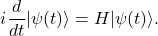
Here,  denotes the state at time
 , and
 is the Hamiltonian. As the total-energy operator, the Hamiltonian determines how that state evolves. Solving the Schrödinger equation with a specified Hamiltonian and initial state gives the state at any later time.
When the Hamiltonian is independent of time, this equation has the formal solution
(4) 
Here,  is the time-evolution operator. Its unitarity preserves the norm of the state, so the total probability remains unchanged as the ideal closed system evolves.
(5) 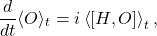
When  , the expectation value of
 stays constant and is conserved. For
 , the expectation value generally changes as the system evolves. We calculate local magnetization, total magnetization, and connected correlations as expectation values of the state after evolution under
 . Their time dependence follows from the commutators above: the local
 and pair
 observables do not commute with the transverse-field term. The explicit commutator derived below also shows which operator combinations allow the transverse field and Ising interaction to generate correlations together.
Integrability, Chaos, and Operator Growth
An integrable many-body model has an extensive set of conserved quantities. These constrain its evolution and allow a description in simpler degrees of freedom3. At hz=0, a Jordan–Wigner transformation maps the transverse-field Ising chain to free fermions5. Interactions, correlations, and information spreading can still appear in the spin dynamics, but the conserved quantities restrict how the state explores Hilbert space.
A nonzero longitudinal field generally breaks this free-fermion description and makes the tilted-field model non-integrable6. Information that was initially accessible through a local observable can then spread across many degrees of freedom, allowing local relaxation and more complicated dynamics. Establishing quantum chaos or thermalization in a finite-time trajectory requires further diagnostics; non-integrability alone does not establish either behavior.
Here we use magnetization and equal-time two-point expectations to benchmark the hardware dynamics. These quantities do not supply the level-spacing statistics, out-of-time-order correlators, or entanglement measurements needed to independently diagnose chaos, thermalization, or operator growth. We therefore compare hz=0 with hz=hx through their measured magnetization and connected correlations. The longer theoretical discussion is given in Supplementary File S1.
The 1D Tilted-Field Ising Model
The Ising model is a standard model in statistical mechanics and condensed matter physics used to study how local spin interactions can produce collective behavior. In the quantum Ising model, spins are represented by Pauli operators, and the dynamics are governed by a Hamiltonian. The tilted-field Ising model is written as14
(6) 
Open boundary conditions are used throughout. For  , the interaction sum therefore contains 14 nearest-neighbor bonds, while each field term acts on all 15 sites. Throughout this work, natural units are used, so
 , and the parameters
 ,
 , and
 are treated as dimensionless simulation parameters that set the relative strengths of the Hamiltonian terms. Here, and
 are Pauli operators acting on site
 , is the nearest-neighbor coupling strength, is the transverse-field strength, and is the longitudinal-field strength. In this study, the computational basis states are identified with the spin states in the
 -basis according to the standard Pauli- convention,

Thus,

Therefore, a qubit in the state has spin-up orientation along the direction, while a qubit in the state has spin-down orientation along the direction. This convention is used when interpreting local magnetization values, so  corresponds to a spin mostly aligned upward along the axis, while
 corresponds to a spin mostly aligned downward along the axis.
The first term,
(7) 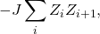
describes the interaction between neighboring spins. For a pair of neighboring spins in a -basis configuration, the measurement outcome of  is
 when the two spins are aligned and
 when they are anti-aligned. Therefore, this term determines whether the system energetically favors aligned or alternating spin configurations. For positive , aligned configurations are favored, which is called ferromagnetic behavior; for negative , alternating configurations are favored, which is called antiferromagnetic behavior14. This term makes the model many-body because the energy of one spin depends on the state of its neighbor.
The second term,
(8) 
represents the transverse field. It is called transverse because it acts in the  direction while spin-up and spin-down are defined along the direction. The operator flips the spin on site , changing into and into . This term introduces quantum fluctuations because it prevents the system from remaining fixed in a single classical spin configuration. It is therefore essential to the quantum dynamics of the transverse-field Ising model.
The third term,
(9) 
represents the longitudinal field. It is called longitudinal because it acts along the same direction as the Ising interaction. This term biases the system toward one spin direction along the axis. A positive longitudinal field favors spin-up states, while a negative longitudinal field favors spin-down states. The longitudinal field is theoretically important because it breaks the integrable structure of the transverse-field Ising model.
Integrable
When
(10) 
the Hamiltonian reduces to the transverse-field Ising model.
Non-Integrable
When
(11) 
the model becomes the tilted-field Ising model. The longitudinal field breaks the free-fermion structure of the transverse-field Ising model and generally makes the system non-integrable. This means the additional conserved structure of the integrable model is lost, allowing more complex many-body dynamics to emerge15.
The dynamics depend on the relative strengths of the interaction and field terms. In the field-dominated limit  , single-site rotations set the leading motion and the weaker spin–spin coupling generally produces correlations more slowly. In the interaction-dominated limit
 , neighboring spins strongly influence one another and the response becomes more collective. The intermediate regime
 contains direct competition between field-driven rotations and interaction-driven organization in the basis, so neither contribution can be neglected.
The six benchmark cases use , 1.0, and 1.4. All three lie near this intermediate scale rather than deep in either asymptotic limit. They are therefore described as lower, matched, and higher coupling cases, not as distinct field- and interaction-dominated phases. Supplementary File S1 retains the extended discussion of these limiting regimes.
Quantum Circuits
A quantum circuit applies an ordered sequence of unitary gates to qubits13. A gate acts on one or more qubits while preserving total probability. To simulate a Hamiltonian digitally, we approximate the continuous evolution by repeating gate layers for its simpler component terms1,2. This gives a circuit that can be executed on the device. The approximation introduces a product-formula error when the components do not commute, as discussed below. Supplementary File S1 gives the fuller introduction to qubits, gates, and digital simulation.
The gates follow from the form of each Hamiltonian term. Exponentiating the transverse-field term involving gives single-qubit rotations about the axis. The longitudinal-field term involving gives rotations about the axis. The interaction term involving acts on neighboring spin pairs, so its exponential requires two-qubit operations.
Hardware Noise in Quantum Circuit Implementation
On quantum hardware, control pulses approximate the intended unitary gates, so coherent over- or under-rotation, unwanted phases, and stochastic gate errors can accumulate with circuit depth4. Two-qubit errors are particularly relevant because the repeated  layers create the nearest-neighbor interactions and correlations being benchmarked. Readout assignment error can flip recorded outcomes and bias both
 and
 , while finite sampling adds estimator variance rather than a deterministic contraction.
Environmental coupling also produces  relaxation and
 dephasing; residual coupling and crosstalk can introduce additional qubit- and layer-dependent errors16. These processes can alter amplitudes, phases, and correlation structure, but the retained archive contains expectation values rather than raw outcomes, covariance, calibration-matched controls, or path-specific calibration records. The observed discrepancies therefore cannot be assigned to one unique hardware-noise mechanism. Supplementary File S1 retains the extended mechanism-by-mechanism discussion.
Trotterization
Trotterization approximates evolution under the full Hamiltonian by applying the simpler component evolutions in sequence17,18. With the signs in Eq. (6), we write  , where
 ,
 , and
 . The two diagonal terms,
 and
 , commute with each other. The transverse term
 generally does not commute with them, and the Baker–Campbell–Hausdorff expansion expresses the resulting splitting error through these commutators19.
Combining the commuting diagonal terms gives the following symmetric second-order step:
(12) 
At  , the product-formula state is
 . In Qiskit’s convention,
 , so each diagonal half-layer uses
 for and
 for
 . The intervening transverse layer uses
 for
 . Symmetric ordering gives a local error of
 and a fixed-time global error of
 19; the convergence test below checks this scaling. Reducing t lowers the splitting error, but requires more gate layers and exposes the state to hardware noise for longer. Supplementary File S1 gives the derivation and the corresponding resource trade-off.
Observables
For the ideal state  obtained from this product formula, we evaluate three observable families:
(13) 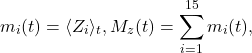
(14) 
Local magnetization gives the polarization at each site; total magnetization sums those values over the chain. Connected correlations remove the product of the two one-site polarizations, leaving the part that cannot be explained by independent measurements. A nonzero value indicates statistical dependence between the measured components, but is insufficient on its own to establish entanglement. We use 15 local components, one derived total, and 14 center-to-site connected components. Full definitions and their physical interpretation appear in the Supplementary Information section “Expanded observable definitions.”
Quantitative Benchmarking Metrics
To quantify hardware–simulation agreement, the IBM hardware data were compared with the noiseless second-order Trotterized simulation at the same  hardware sampling times. Let
 and
 denote the hardware and ideal Trotter values, respectively, for component
 of observable at sampled time
 8,9,10. Hardware data were not interpolated. The pooled raw root-mean-square error was defined as
(15) 
Because the three observable families have different natural scales and component counts, raw RMSE is compared within rather than across families.
Small connected-correlation amplitudes make an all-zero output an important baseline. Zero-baseline skill was defined as
(16) 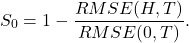
A positive value means that the hardware trajectory is closer to the ideal trajectory than an all-zero predictor; a nonpositive value means that it is not. This baseline prevents a small raw error from being interpreted as faithful dynamics when the target signal is itself close to zero. Temporal shape was assessed component-wise using Pearson coefficients and Fisher- averaging. An empirical exponential-contraction fit and circular moving-block sensitivity analysis are reported in Supplementary File S1. These are trajectory diagnostics, not experimental confidence intervals. For 2048 independent direct Pauli measurements,  , but connected correlations and total magnetization require unavailable covariance information. The breakdown-time statistic is retained in S1 only as a threshold-sensitivity diagnostic.
Numerical and Hardware Methods
Trotterization Procedure
The tilted-field Ising Hamiltonian cannot be implemented as one single operation in a gate-based quantum circuit, so it must be decomposed into simpler pieces that can be applied sequentially. For the tilted-field Ising Hamiltonian, the relevant positive generators used for the circuit decomposition are the -dependent generator,

and the transverse-field generator,
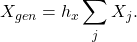
Using the Pauli commutation relation  and the standard product identity
 , the commutator becomes
(17) 
This commutator shows that the transverse field does not act independently of the -dependent terms. The transverse field flips spins, while the Ising interaction and longitudinal field align neighboring spins and bias them along the direction. Since these effects do not commute, they generate new operator structures involving  and neighboring combinations such as
 and
 . These structures show how local spin flips become linked to neighboring spin configurations, providing a way for connected correlations to form between sites.18. In this simulation, the relevant dimensionless factors are

The second-order error depends on commutators and nested commutators, not on a universal rule that each bare parameter must be below one. Accuracy was therefore established directly through exact sparse matrix-exponential-action validation and fixed-H timestep convergence rather than inferred from parameter magnitude alone.
The six base cases used ; or  ; and
 , , or
 . The transverse field was fixed so that the comparison focused on the longitudinal field and nearest-neighbor interaction.
The cases act as the transverse-field Ising reference set, while the  cases show how the selected observables change after the tilted field is introduced. The parameter values were fixed before the archived hardware execution after approximately 250 exploratory development simulations. The outputs and numerical selection rule from that preliminary scan were not archived and therefore cannot now be reconstructed or quantitatively assessed. Because selecting cases for stable late-time behavior could favor trajectories for which decoherence produces apparent agreement with a small ideal signal, the preliminary scan is treated as a possible source of selection bias rather than as evidence for the benchmark conclusions. The six cases are therefore interpreted as an exploratory parameter set rather than a representative sweep of parameter space.
Second-order symmetric Trotterization was used with timestep

This timestep provided a manageable circuit depth while still allowing the dynamics of the model to be resolved. Its accuracy was assessed against exact sparse matrix-exponential-action evolution for local magnetization, total magnetization, and all 14 center-to-site connected correlations in all six base cases. Across those cases, exact-versus-product-formula RMSE ranges from  to
 for local magnetization and from
 to
 for total magnetization; the largest connected-correlation RMSE is
 . A fixed-H test at
 , 0.10, and 0.05 gives fitted global-error slopes of 2.002, 2.005, and 2.001 for the three observable families, consistent with a symmetric second-order product formula whose local one-step error scales as 20. Complete residuals and convergence tables are reported in the Supplementary Information. The
 parameter calculation in Figure 1(b) is retained as a stress test, not a timestep-convergence test, because it changes the Hamiltonian while holding
 fixed.
Finally, the Trotter timestep was fixed at  for the IBM quantum hardware implementation. The selected backend was
 . To reduce the total hardware runtime while preserving the same Trotterized dynamics, IBM hardware observables were sampled every
 units of evolution time. The IBM hardware circuits were run with 2048 shots per circuit. Circuits were transpiled with optimization level 0. This level still performs layout, routing, and basis translation and therefore does not guarantee that the logical Trotter-layer structure is preserved on the device. The historical transpiled circuits were not archived, so native gate counts, two-qubit depth, duration, routing overhead, and calibration-weighted error cannot be reconstructed. The simulation curves were evaluated on the grid, while hardware results are shown at the 71 sampled times. At finite , the repeated layers also define a discrete Floquet evolution whose deviations from continuous-time dynamics are quantified by the exact and fixed-H checks above7.
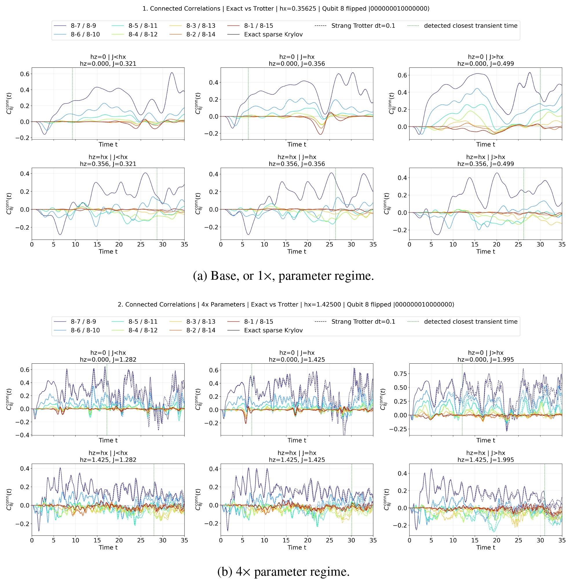
 . Subfigure (a) uses the base parameters of the hardware benchmark. Subfigure (b) multiplies , , and by four at fixed and is a stress test rather than a convergence test. Each subfigure contains the six parameter cases, with
 in the top row,
 in the bottom row, and , 1.0, and 1.4 across columns. Mirror-related curves overlap because the uniform open Hamiltonian and centered initial state are reflection symmetric. The dashed green line is the closest transient-stability time used when generating the original plots; it is not used as a fidelity metric in this revision. Numerical errors for all three observable families and a fixed-H timestep-convergence test are reported in the Supplementary Information
In the base calculation, the exact and Trotterized connected-correlation curves remain closely aligned across all six cases, with maximum RMSE . The calculation shows more noticeable separation because the Hamiltonian scale is changed at fixed timestep. It therefore demonstrates a higher-scale stress condition but does not establish convergence with respect to . The separate fixed-H study establishes the expected global second-order scaling. Together, these checks separate the small product-formula error of the base reference from the much larger hardware discrepancy.
Circuit Implementation
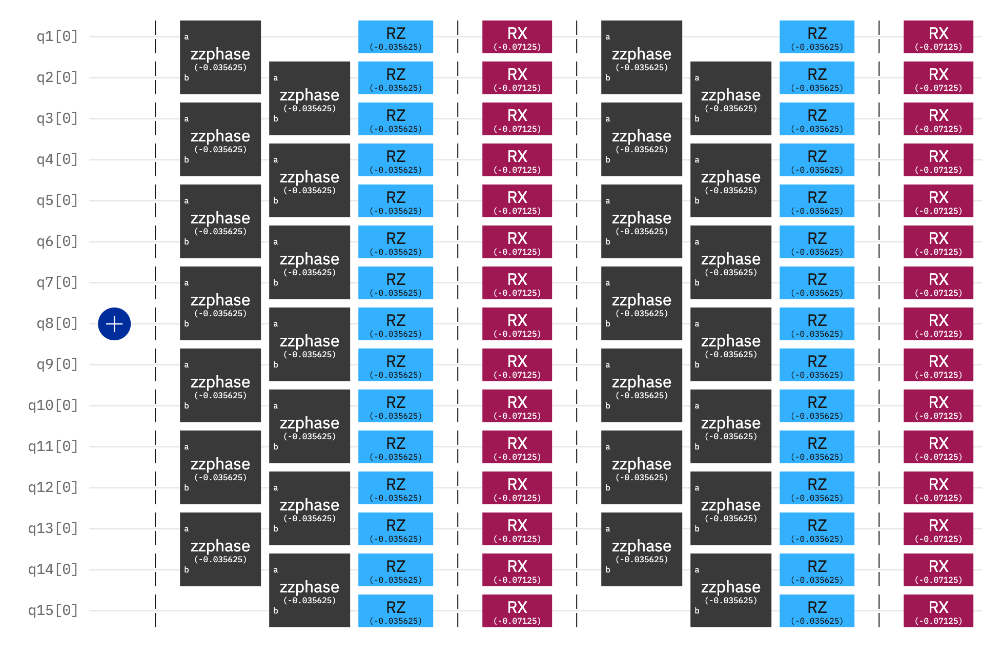 ,
 case. An gate prepares site 8 in while all other sites remain in . The complete step is
 : each diagonal half-layer contains nearest-neighbor zzphase and one-site rotations, and the central layer contains rotations. In Qiskit’s gate convention the displayed half-step angles are
 and
 , while the full transverse angle is
 . The original image is retained; its terminal preview of the following repeated block is cropped so that the displayed unit ends after the second diagonal half-layer.
The Qiskit convention for the two-qubit rotation is22
(18) 
For the interaction Hamiltonian  , the diagonal half-step
 uses the Qiskit angle
 , rather than
 , because the gate definition already includes the factor of one half. The longitudinal half-step uses
 , and the full transverse step uses
 . These layers give the symmetric sequence .
Each qubit represents one site of the spin chain. We prepared the chain with all spins up except the central qubit,  , which was flipped down. Starting with every qubit in the computational basis state , we applied an gate to the eighth qubit. The resulting state of the 15-qubit system is

The central spin flip lets us examine how a localized excitation affects site-resolved magnetization and center-to-site correlations over time.
We implemented each term of Eq. (6) through its corresponding time-evolution operator. The initial Pauli- gate creates the spin-down excitation before this evolution begins. A diagonal half-step applies  using nearest-neighbor rotations and one-site rotations. The central layer applies
 through rotations. Repeating the complete symmetric step 350 times gives the trajectory up to .
Reproducibility details
All hardware circuits were executed on the IBM backend ibm_marrakesh. The hardware data were collected on May 16, 2026. The aggregate backend values reported in supplementary file S1 describe the run period but are not a calibration record for the unknown physical 15-qubit path. The circuits were run without user-implemented postselection or full quantum error correction. In the archived hardware-submission code, IBM Runtime EstimatorV2 was configured with resilience_level = 1, and dynamical decoupling was requested using the XpXm sequence. No additional user-implemented zero-noise extrapolation, postselection, or custom measurement-error mitigation was applied. Because per-job Runtime metadata were not preserved in the stored cache, the realized settings cannot be independently reconfirmed from the archived expectation-value arrays alone.
Exact trajectories used scipy.sparse.linalg.expm_multiply; numerical checks included state-norm preservation and observable convergence23. Qiskit’s little-endian mapping was applied consistently. Six cases at 71 times produced 426 circuits, each requested with 2048 shots and optimization level 0. The saved array contains 15 local and 14 pair expectations per case and time. Raw outcomes, covariance, complete Runtime metadata, layouts, historical transpiled circuits, and path-specific calibration snapshots were not retained. The full software versions, string-indexing rule, archive shape, and logical-resource counts remain in the Supplementary Information under “Reproducibility and archived resources.”
Results
Exact Validation of the Ideal Product Formula
In all six base cases, the exact-versus-product-formula errors reported above are much smaller than the hardware discrepancies. The fixed-H convergence slopes are close to two, as expected for global second-order behavior. Figure 1 shows the original connected-correlation comparison. The Supplementary Information gives the numerical residuals for local magnetization, total magnetization, and all 14 connected correlations.
Local Magnetization
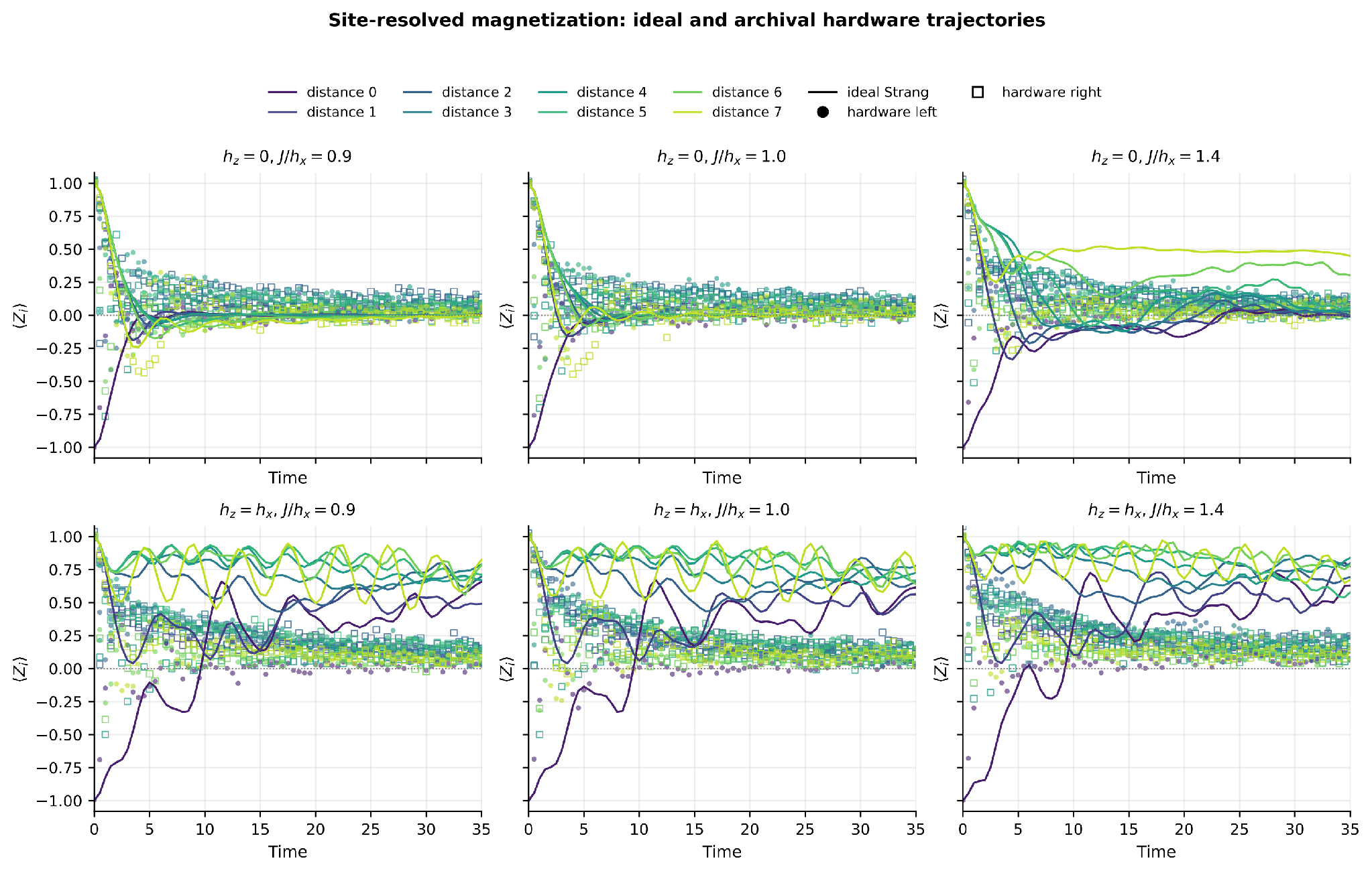
All six hardware cases in Figure 3 have lower RMSE than the all-zero trajectory, with zero-baseline skill between 15.4% and 27.8%. The agreement in time still varies across sites. For , the ideal  curves change rapidly at early times and then approach values close to zero at most sites. Strong early oscillations are especially visible for and 1.0. At , several qubits keep a larger positive magnetization for longer, leaving the curves more separated and slowing their approach toward zero.
In the bottom row, , many ideal local-magnetization curves remain positive through most of the plotted interval. Several stay between roughly and  , particularly for and 1.4, rather than approaching zero. The positive longitudinal field favors
 alignment and accounts for this stronger polarization. That bias alone provides no evidence for quantum chaos or thermalization.
The hardware data also show an early decrease in magnetization, but their amplitudes span a smaller range than the ideal curves. For , most hardware values lie near zero after the initial drop and broadly follow the scale of the ideal response. The separation is larger for : the ideal simulation keeps higher local magnetization, while the hardware values are lower and vary less from site to site. We quantify this loss of amplitude with the contraction analysis below. The fit describes the discrepancy without identifying a single noise mechanism.
Total Magnetization
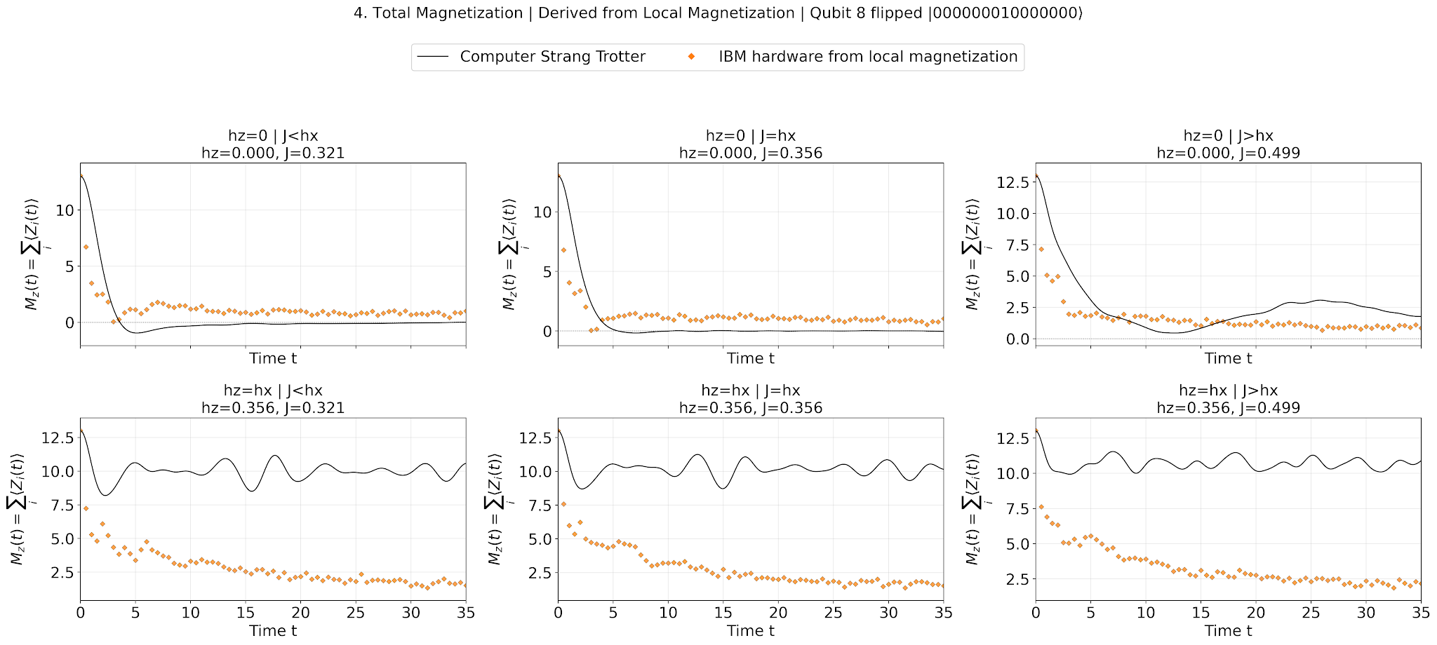
 for the six parameter cases. The black curves show the ideal second-order Trotter simulation, while the orange markers show IBM hardware totals obtained by summing the same 15 local expectations in Figure 3. The prepared state has
 . Rows distinguish and 1; columns show , 1.0, and 1.4. Total magnetization is a derived aggregation rather than an independent hardware circuit family, and its sampling uncertainty depends on covariance among the local estimates, which was not saved.
Figure 4 compares the collective magnetization of the ideal and hardware trajectories. All six hardware trajectories outperform the zero predictor, with zero-baseline skill of 36.6–52.6% for and 27.0–30.6% for . In the cases, the ideal simulation begins at 13 and then drops sharply at early times. For and 1.0, the ideal total magnetization falls close to zero after the initial transient and remains near zero for most of the plotted window. In the case, it also decreases early but retains a larger positive value during parts of the evolution.
The hardware values in the row also decrease quickly from the initial value. After the early-time drop, they remain low and relatively stable but do not reproduce the detailed temporal structure of the ideal simulation. For and 1.0, the hardware total settles slightly above zero while the ideal trajectory remains closer to zero. For , both trajectories remain positive after the initial decrease, although their later-time structures differ.
The cases show a larger difference between the ideal simulation and hardware. In the ideal trajectories, total magnetization decreases initially but remains positively polarized, whereas the hardware total is substantially contracted. The zero-baseline results nevertheless show that the hardware retains nontrivial collective information in all six cases, without implying faithful reproduction of the full many-body state.
Signed Site-Resolved Center-to-Site Connected Correlations
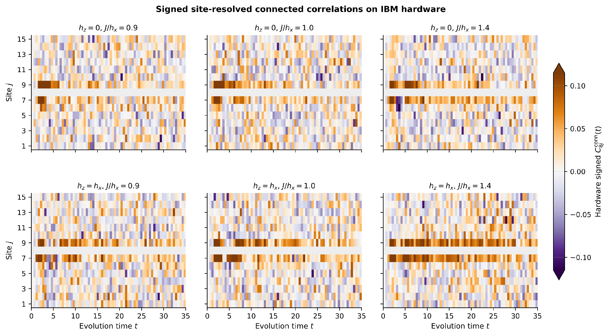
Figure 5 shows the signed hardware center-to-site connected-correlation maps for all six cases. The corresponding ideal signed maps are provided in Supplementary File S1. In the ideal simulation, the center-to-site correlations develop through the combined noncommuting transverse-field and nearest-neighbor interaction dynamics. The diagonal  interaction alone commutes with each local and therefore cannot generate the observed -basis correlation dynamics from the initial computational-basis product state. The uniform open Hamiltonian and centered initial state also preserve reflection symmetry about site 8, as confirmed numerically in the Supplementary Information.
The connected-correlation benchmark gives a different result from the magnetization observables. Four of the six hardware cases fail to outperform an all-zero trajectory, while the remaining two improve over zero by only 2.9% and 0.8%. Their comparatively small absolute RMSE therefore does not establish faithful reproduction of the ideal correlation dynamics when the ideal signal itself is small.
The archived hardware data also do not retain the covariance required to determine uncertainty in  . Consequently, isolated nonzero hardware values are not treated as statistically resolved correlations, and no hardware first-arrival time or propagation velocity is claimed.
Quantitative Benchmarking of Hardware–Simulation Agreement
To move beyond visual comparison, agreement between the IBM hardware results and the ideal second-order Trotter simulation was quantified using the raw RMSE, zero-baseline skill, Fisher- temporal-correlation summaries, and the empirical contraction model defined above. The complete 18-row RMSE and zero-baseline-skill table is reported in Supplementary File S1. The main findings and numerical ranges are stated below.
For scale, 2048 independent direct Pauli shots correspond to a single-expectation standard-error upper bound of approximately  . Because the archived Runtime outputs do not retain the raw measurement outcomes, covariance information, or returned Estimator uncertainties, this value is used only as a nominal sampling scale and not as an experimental error bar on the reported metrics.
Local magnetization outperformed the all-zero trajectory in every case, with  between 15.4% and 27.8%. Total magnetization also outperformed zero in every case, with between 27.0% and 52.6%. These results show partial retention of nontrivial magnetization-scale information under the selected RMSE metric, while making no claim of state fidelity.
Connected correlations produced a different result. The hardware failed to outperform zero in four of the six cases. In the other two cases, improvement over zero was only 2.9% for , and 0.8% for , . Their comparatively small absolute RMSE therefore does not indicate faithful reproduction when the ideal signal itself is small.
Fisher- mean temporal correlations for local magnetization are 0.694–0.746 for and 0.402–0.459 for . Individual-site values are heterogeneous: the minimum reaches  , the maximum reaches 0.959, and the central-site values range from 0.294 to 0.578. For connected correlations, none of the six cases provides evidence of positive temporal agreement under the seven-sample-block diagnostic: four intervals include zero, while the , interval is narrowly negative at
 and the , interval is negative at
 . These intervals are conditional trajectory-shape diagnostics rather than experimental confidence intervals.
The contraction model reduces pooled local-magnetization RMSE by 18–49% for and by 67–68% for . Fitted  values range from 0.572 to 1.022 and from 0.104 to 0.128, respectively. Residual discrepancy remains, so a scalar contraction does not fully explain the data and is not identified with a unique noise process. Complete component statistics, block-length sensitivity, contraction intervals, signed correlation maps, logical resource counts, and breakdown-threshold sensitivity are reported in the Supplementary Information.
Discussion
Hamiltonian Dynamics
The cases provide the transverse-field Ising reference. Here the transverse field and nearest-neighbor Ising interaction determine the dynamics, with no longitudinal bias. For and 1.0, Figures 3 and 4 show a rapid early decrease in local and total magnetization, and most qubits approach values near zero. This is consistent with the transverse field rotating the spins away from the measured basis. At , several sites stay more positively polarized for longer. The higher selected coupling therefore changes the magnetization response of this finite chain. These three cases do not represent asymptotic field-dominated or interaction-dominated limits.
The lower row, , shows how a longitudinal field changes the response. Figures 3 and 4 show stronger ideal local and total magnetization than in the corresponding cases. This field acts along the measured direction and favors positive -axis polarization. Meanwhile, the transverse field rotates spins away from the basis, and the interaction couples neighboring sites. The competing terms produce oscillations instead of a steady approach toward zero, especially for and 1.4. The longitudinal bias explains the contrast between rows without requiring an interpretation in terms of chaos or thermalization.
Interpreting the six hardware panels in Figure 5 also requires the ideal correlation maps. Those correlations develop through the noncommuting transverse-field and interaction dynamics: the interaction alone is diagonal in the measurement basis and commutes with each local . Reflection about site 8 leaves both the uniform open chain and the central spin flip unchanged. The mirror-related ideal curves consequently overlap to about  or better in every case. Increasing
 broadens the correlation pattern in this finite chain, while later bands also contain interference and boundary reflections. The ideal signed maps in the Supplementary Information distinguish positive from negative structure. We extract no propagation velocity from the hardware data.
Ideal Simulation vs Hardware
Figure 3 shows that ibm_marrakesh reproduces part of the early magnetization response. The initially upward spins move away from their starting values, while the flipped central spin begins in the opposite state. Both features are visible in the ideal and hardware trajectories. The hardware curves, however, cover a smaller range and separate less clearly across sites. For , they outperform the all-zero predictor by 15.4–19.8%. Across all six cases, that improvement ranges from 15.4–27.8%. The local signal thus contains information beyond zero in both field settings, even though its temporal pattern is only partly reproduced. The component-wise correlations make this distinction clear: temporal agreement differs substantially from one site to another, so the positive skill values do not establish full temporal fidelity.
The exponential-contraction fit describes part of this amplitude loss. It reduces pooled local-magnetization RMSE by 18–49% for and 67–68% for , without isolating the physical source. Readout bias, coherent and stochastic gate errors, relaxation, dephasing, routing, crosstalk, and backend processing could all contribute. The saved expectations cannot separate them. In the Supplementary Information, the seven logical mirror-site pairs provide a second check that does not depend on an ideal reference trajectory. Ideal evolution preserves reflection symmetry to numerical precision; the hardware has overall mirror-asymmetry RMS values of 0.117–0.167. This asymmetry is strongest early in the evolution and is especially pronounced for the pair at logical sites 4–12. Without the physical layout, we cannot associate it with particular device qubits or couplers. Finite-shot sampling adds variance, but cannot alone explain a systematic contraction. In the adopted convention, relaxation toward would increase at the fourteen initially upward sites. It therefore cannot by itself account for the observed downward amplitude shift.
The discrepancy is larger for . Several ideal site trajectories retain positive polarization and oscillations as the three Hamiltonian terms compete, but the hardware reproduces these features less accurately. The Fisher- mean temporal correlations fall from 0.694–0.746 for to 0.402–0.459 for . Individual components span a broad range, with central-site values from 0.294 to 0.578. These numbers describe a difference in the measured observables for the selected circuits. They do not justify attributing the difference to chaos or to a particular decoherence channel.
Total magnetization in Figure 4 follows a similar pattern. The ideal total changes rapidly at early times and stays positive in the tilted-field cases, retaining memory of the initial -basis polarization. The hardware total is lower and moves closer to zero. Its zero-baseline skill nevertheless reaches 36.6–52.6% for and 27.0–30.6% for . Every total-magnetization trajectory therefore contains a collective signal that improves on zero. Four of the six connected-correlation trajectories fail the same comparison.
Because total magnetization sums every local expectation, its numerical scale differs from that of one site or a connected pair. We therefore compare raw RMSE within each observable family, rather than across families. Uncertainty in the total also depends on covariance between the local estimates, which cannot be reconstructed from the saved expectations. Readout bias, gate imperfections, and errors in the programmed interaction layers may each shift the measured total. The archive does not allow their individual contributions to be separated.
The ideal signed maps in Supplementary File S1 resolve the center-to-site correlations as they evolve under the noncommuting transverse field and nearest-neighbor interaction. The strongest features remain around site 8. Later bands also contain interference within the finite chain and reflections from its boundaries. We found no statistically resolved first-arrival front in the hardware data, so these finite-chain results provide no estimate of a hardware propagation velocity.
The IBM hardware panels have weaker structured contrast and more isolated nonzero pixels. Four connected-correlation cases fail to outperform the all-zero trajectory; the other two improve on it by only 2.9% and 0.8%. Their small absolute RMSE must be read alongside the small ideal signal: it does not demonstrate recovery of the temporal pattern. The primary conditional moving-block intervals include zero in four cases and are negative in two, including the , case.
A connected correlation is calculated from  , so errors in the joint expectation and in either local expectation enter the final value. These estimates are also statistically correlated. The finite-shot bound for a directly measured Pauli expectation, given in Methods, cannot supply an uncertainty bar for this combined quantity. That calculation would require a bitstring bootstrap or a delta method that includes covariance. Raw outcomes were not saved, so neither can be carried out on this archive. The isolated nonzero hardware pixels consequently do not resolve a propagation front.
Supplementary File S1 gives the threshold-dependent agreement-breakdown analysis. With the original definition, local and total magnetization both gave  . The connected-correlation values ranged from 2.0 to 24.5 at threshold 0.05, while every case was right-censored beyond 35 at threshold 0.15. The inferred time changes with the threshold, the required persistence, and the signal scale. These dependencies prevent interpreting
 as a measure of fidelity.
The hardware retains different amounts of information in the three observable families. Total magnetization gives the strongest improvement over the zero baseline. Local magnetization preserves some site-resolved behavior, with substantial variation between sites, while the connected correlations provide little reliable separation from a zero output. A collective response can therefore survive even when the weaker multicomponent correlations are poorly reproduced. This conclusion applies to the backend, execution period, initial state, system size, parameter cases, and circuit implementation examined here.
The archive cannot establish whether error mitigation improved these measurements. Our submission code requested Runtime resilience level 1 and XpXm dynamical decoupling, but the complete returned metadata were not saved. We did not run mitigation-off, dynamical-decoupling-off, or calibration-matched noisy-simulator controls. Although mitigation may improve future hardware estimates, it needs a controlled comparison in this setting. Future runs should define those control arms in advance and retain the raw counts, physical layouts, transpiled circuits, calibration snapshots, and repeated executions24,25,26.
Supplementary File S1 gives the recommendations for measurement order and native depth, the covariance information needed for connected correlations, and the full discussion of fault-tolerant overhead.
Conclusion
This archived 15-qubit tilted-field Ising execution preserved part of the magnetization response, but did not establish faithful center-to-site connected-correlation dynamics. Exact sparse evolution and the fixed-Hamiltonian convergence test validate the ideal second-order reference. Every local- and total-magnetization case improves on the zero baseline. Four connected-correlation cases do not, and the other two improve by only 2.9% and 0.8%. The contraction fit and symmetry checks describe aspects of the hardware discrepancy; they neither identify a unique noise mechanism nor demonstrate successful reconstruction of the ideal dynamics.
These findings concern one initial state, chain size, backend, execution period, and six selected parameter cases. The archive lacks returned per-job settings, raw outcomes, covariance, repeated executions, physical layouts, historical transpiled circuits, and calibration records for the physical path. Future experiments should save these records, fix or record that path, repeat representative circuits across calibration windows, and compare runs with controlled mitigation and dynamical decoupling. Supplementary File S1 retains the full account of the limitations and proposed follow-up work, including smaller-chain controls and additional diagnostics of chaos or operator spreading.
Code and Data Availability. Analysis code and archived processed data: GitHub repository.
Supplementary Information
References
- S. Lloyd. Universal quantum simulators. Science. Vol. 273, pg. 1073–1078, 1996, https://doi.org/10.1126/science.273.5278.1073. [↩] [↩]
- A. M. Childs, D. Maslov, Y. Nam, N. J. Ross, Y. Su. Toward the first quantum simulation with quantum speedup. Proceedings of the National Academy of Sciences. Vol. 115, pg. 9456–9461, 2018, https://doi.org/10.1073/pnas.1801723115. [↩] [↩]
- L. D’Alessio, Y. Kafri, A. Polkovnikov, M. Rigol. From quantum chaos and eigenstate thermalization to statistical mechanics and thermodynamics. Advances in Physics. Vol. 65, pg. 239–362, 2016, https://doi.org/10.1080/00018732.2016.1198134. [↩] [↩]
- J. Preskill. Quantum computing in the NISQ era and beyond. Quantum. Vol. 2, pg. 79, 2018, https://doi.org/10.22331/q-2018-08-06-79. [↩] [↩]
- P. Pfeuty. The one-dimensional Ising model with a transverse field. Annals of Physics. Vol. 57, pg. 79–90, 1970, https://doi.org/10.1016/0003-4916(70)90270-8. [↩] [↩]
- J. Karthik, A. Sharma, A. Lakshminarayan. Entanglement, avoided crossings, and quantum chaos in an Ising model with a tilted magnetic field. Physical Review A. Vol. 75, pg. 022304, 2007, https://doi.org/10.1103/PhysRevA.75.022304. [↩] [↩]
- Y. Kim, A. Eddins, S. Anand, K. X. Wei, E. van den Berg, S. Rosenblatt, H. Nayfeh, Y. Wu, M. Zaletel, K. Temme, A. Kandala. Evidence for the utility of quantum computing before fault tolerance. Nature. Vol. 618, pg. 500–505, 2023, https://doi.org/10.1038/s41586-023-06096-3. [↩] [↩]
- P. M. Poggi, N. K. Lysne, K. W. Kuper, I. H. Deutsch, P. S. Jessen. Quantifying the sensitivity to errors in analog quantum simulation. PRX Quantum. Vol. 1, pg. 020308, 2020, https://doi.org/10.1103/PRXQuantum.1.020308. [↩] [↩]
- A. Miessen, D. J. Egger, I. Tavernelli, G. Mazzola. Benchmarking digital quantum simulations above hundreds of qubits using quantum critical dynamics. PRX Quantum. Vol. 5, pg. 040320, 2024, https://doi.org/10.1103/PRXQuantum.5.040320. [↩] [↩]
- E. Granet, H. Dreyer. AppQSim: application-oriented benchmarks for Hamiltonian simulation on a quantum computer. Physical Review Research. Vol. 7, pg. 043146, 2025, https://doi.org/10.1103/qt55-7d6r. [↩] [↩]
- D. J. Griffiths, D. F. Schroeter. Introduction to quantum mechanics. 3rd ed., Cambridge University Press, 2018. [↩] [↩]
- J. J. Sakurai, J. Napolitano. Modern quantum mechanics. 2nd ed., Cambridge University Press, 2017. [↩] [↩]
- M. A. Nielsen, I. L. Chuang. Quantum computation and quantum information. 10th anniversary ed., Cambridge University Press, 2010. [↩] [↩]
- S. Sachdev. Quantum phase transitions. 2nd ed., Cambridge University Press, 2011. [↩] [↩]
- F. Haake, S. Gnutzmann, M. Kuś. Quantum signatures of chaos. 4th ed., Springer, 2018, https://doi.org/10.1007/978-3-319-97580-1. [↩]
- P. Murali, D. C. McKay, M. Martonosi, A. Javadi-Abhari. Software mitigation of crosstalk on noisy intermediate-scale quantum computers. Proceedings of the Twenty-Fifth International Conference on Architectural Support for Programming Languages and Operating Systems. pg. 1001–1016, 2020, https://doi.org/10.1145/3373376.3378477. [↩]
- H. F. Trotter. On the product of semi-groups of operators. Proceedings of the American Mathematical Society. Vol. 10, pg. 545–551, 1959, https://doi.org/10.2307/2033649. [↩]
- M. Suzuki. General theory of fractal path integrals with applications to many-body theories and statistical physics. Journal of Mathematical Physics. Vol. 32, pg. 400–407, 1991, https://doi.org/10.1063/1.529425. [↩] [↩]
- A. M. Childs, Y. Su, M. C. Tran, N. Wiebe, S. Zhu. Theory of Trotter error with commutator scaling. Physical Review X. Vol. 11, pg. 011020, 2021, https://doi.org/10.1103/PhysRevX.11.011020. [↩] [↩]
- G. Strang. On the construction and comparison of difference schemes. SIAM Journal on Numerical Analysis. Vol. 5, pg. 506–517, 1968, https://doi.org/10.1137/0705041. [↩]
- IBM Quantum. IBM Quantum Composer. https://quantum.cloud.ibm.com/composer, accessed May 8, 2026. [↩]
- IBM Quantum. RZZGate. Qiskit API documentation. https://quantum.cloud.ibm.com/docs/en/api/qiskit/qiskit.circuit.library.RZZGate, accessed October 12, 2026. [↩]
- A. H. Al-Mohy, N. J. Higham. Computing the action of the matrix exponential, with an application to exponential integrators. SIAM Journal on Scientific Computing. Vol. 33, pg. 488–511, 2011, https://doi.org/10.1137/100788860. [↩]
- S. Endo, Z. Cai, S. C. Benjamin, X. Yuan. Hybrid quantum-classical algorithms and quantum error mitigation. Journal of the Physical Society of Japan. Vol. 90, pg. 032001, 2021, https://doi.org/10.7566/JPSJ.90.032001. [↩]
- K. Temme, S. Bravyi, J. M. Gambetta. Error mitigation for short-depth quantum circuits. Physical Review Letters. Vol. 119, pg. 180509, 2017, https://doi.org/10.1103/PhysRevLett.119.180509. [↩]
- E. van den Berg, Z. K. Minev, A. Kandala, K. Temme. Probabilistic error cancellation with sparse Pauli–Lindblad models on noisy quantum processors. Nature Physics. Vol. 19, pg. 1116–1121, 2023, https://doi.org/10.1038/s41567-023-02042-2. [↩]