Tuning Hyperparameters to Improve Average Precision in Object Detection for the Nasal Mucosa Cell Dataset

Abstract

Introduction: Nasal cytopathology is an emerging tool to evaluate patient cells and aid diagnoses. Computer vision has the potential to automate counting of cytotype prevalence from cell stain images, increasing efficiency, accuracy, and access. 
Objectives: The primary objective was to evaluate the effects of several hyperparameters on model performance, and the secondary objective was to develop a high-performing model for detecting and classifying nasal mucosa cells.
Methods: The model was developed by tuning data augmentation and loss function hyperparameters, generally by conducting ablation trials over multiple values and selecting values based on mAP50-95. The final models were configured using the chosen hyperparameter values from ablations and were tested using 5 random seeds.
Results: The baseline model scored 0.482±0.021 mAP50 and 0.283±0.012 mAP50-95. The final model scored 0.552±0.019 mAP50 and 0.321±0.010 mAP50-95, corresponding to improvements of 14.5% and 13.4%, respectively.
Conclusions: Specialized hyperparameter tuning yielded moderate improvements in model performance. However, the limited dataset may have hindered the effectiveness of oversampling techniques and data augmentations used in this study. Fundamental changes such as a specialized nasal cytology architecture beyond the general YOLOv12 model, collecting more data and providing patient diagnosis labels, and using larger, more powerful models may be necessary for advancing nasal mucosa cell object detection models.

Keywords: machine learning; object detection; computer vision; nasal cytology; YOLO; chronic rhinosinusitis with nasal polyps

Introduction

Chronic rhinosinusitis with nasal polyps (CRSwNP) is a nasal disease affecting millions of individuals worldwide that may benefit from advances and AI assistance in nasal cytology. CRSwNP is associated with asthma, frequently requires multiple surgeries or therapy with medication, and leads to lower quality-of-life¹.

Cytopathology, the growing field of studying cells under microscopes to reach informed diagnoses and treatments, has multiple advantages, including faster results, cost-effectiveness, and less invasive sampling. Despite these advantages, expertise is still required in interpreting samples, and improper preparation and poor communication between professionals leads to incorrect diagnoses². Early solutions such as the PAPNET and ThinPrep systems demonstrated the upward trajectory of computer-vision-powered cytology³. Leveraging automatic AI in diagnostic processes to assist specialized doctors could help increase patient diagnosis rates and accuracy by reducing time spent for both doctors and patients in diagnoses.

A study conducted on patients diagnosed with CRSwNP subtyped them based on eosinophil cell count. Its experiments found that eosinophil count from nasal cytology on the nasal polyp roughly matched numbers from obtaining surgical samples and those numbers effectively distinguished between subtypes, indicating that nasal cytology can inform patient treatment¹.

Zhang et al.⁴ introduced the quantitative assessment for nasal inflammatory cytology (QANIC) system, which recognizes cell-like objects, distinguishes impurities from cells, and identifies eosinophils and neutrophils, grouping the other cells into a miscellaneous category. Their experiments demonstrated that using QANIC’s output to calculate nasal eosinophil prevalence and using blood work to calculate blood eosinophil prevalence effectively phenotypes chronic rhinitis patients. Its major limitation is that it only counts 2 cytotypes, leaving out others that could provide additional context and prove useful to phenotyping⁴.

Advances in deep learning and object detection provide an opportunity to advance nasal cytology automation, which, in turn, will enable the scaling of nasal cytology and specialized nasal disease and infection treatment. The existing Nasal Mucosa Cell Dataset (NMCD) is small and has imbalanced classes, and the YOLOv8⁵ model published with it scored a mean average precision at threshold 0.5 (mAP50) of 0.478 and at thresholds 0.5 to 0.95 (mAP50-95) of 0.266^6,7, unsuitable for clinical implementation.

Objectives

This study, in an effort to build upon the NMCD and lay the groundwork for future nasal mucosa object detection work, had two objectives. The primary objective was to evaluate the individual effects of several hyperparameters on model performance, providing insight into the most beneficial adjustments for optimizing object detection models on the nasal mucosa cell detection and classification task. The secondary objective was to develop a high-performing model, measured with average precision, using the NMCD for detecting and classifying nasal mucosa cells, building upon the baseline model developed by the NMCD authors⁶.

Limitations

Google Colaboratory (Colab), an online web-based service that connects to GPU runtimes for a small cost, was used for all model training to limit expenses. Colab has usage limits which limited the quantity and intensity of trials that could be performed during model development. Additionally, the NMCD is small and imbalanced, with a total of 500 images and with 4 out of the 10 classes having under 100 training instances. Due to computational limits and small NMCD validation dataset size⁶, this work is exploratory in nature.

Computer vision in medicine

Deep learning advances, hardware improvements, and big data availability have enabled breakthroughs in computer vision tasks, which are especially applicable in medicine. For example, object detection applied to repeated structures in microscope data, such as nasal mucosa cells, can become more accurate and precise than human vision and automate the common routine task of finding and counting such structures⁸.

In 2015, Ronneberger et al.⁹ introduced the revolutionary U-Net, designed for medical image segmentation tasks such as finding cells. The model is characterized by a U-shaped architecture that combines fine, low-level features from the first half of the network with overarching, high-level features from the last half for more detailed context. The U-Net authors also took advantage of translation, rotation, and distortion data augmentations. The trained U-Net model outperformed state-of-the-art in segmenting brain tumor cells, HeLa cells, and brain components⁹.

Archit et al.¹⁰, building upon previous work applying the Segment Anything¹¹ vision foundation model, a large model designed for general computer vision tasks, to medicine, introduced Segment Anything for Microscopy, which created a procedure for retraining and specializing Segment Anything for light microscopy and for electronic microscopy. They also created a user-facing application that performed both human-in-the-loop and computer-driven biomedical image segmentation, marking an advancement in the application of medical microscopy image segmentation¹⁰.

Object detection and YOLOv12

A subset of deep learning and computer vision, object detection locates objects of interest in an image by drawing bounding boxes, the smallest rectangle that encapsulates the object, around them (localization) and classifies such objects (classification)¹². Aggregating such model-generated predictions can calculate totals of each class for each image sample, effectively creating a cytotype distribution when applied to nasal mucosa cells.

The YOLO series of object detection architectures uses a one-stage approach. It is fast and generalizes to new data well. However, it requires lots of data to learn features, similarly to other large object detection models, and does not perform well with overlapping or small objects of interest¹³.

This paper used YOLOv12, the latest architecture in the YOLO object detection series at the start of this paper’s writing; YOLO26 was released a few months after¹⁴. YOLOv12’s primary contribution is its usage of attention, an existing technique which processes context from large regions of the image simultaneously to enhance the model’s understanding¹⁵. In computer vision, attention’s complexity is proportional to the input size squared, but by using the authors’ area attention mechanism, which focuses on a group of contiguous rows or columns, the attention approach is sped up by a factor of 4, making it feasible to implement. YOLOv12 outperformed previous YOLO iterations on the Common Objects in Context (COCO) dataset, a standard benchmark for general-purpose object detection models, while maintaining similar or superior computational efficiency^16,17,18.

YOLO applied to medicine

Ragab et al.¹³ conducted a systematic review of articles applying YOLO to healthcare. They found that YOLO is useful in the field for its ability to detect lesions and other abnormalities correlated to cancer, heart diseases, and other such conditions. Safdar et al.¹⁹ applied YOLOv3 to detecting brain tumors, comparing effectiveness of various data augmentations on improving performance. The 180-degree rotation augmentation performed the highest, with an accuracy of 96%. Chen et al.²⁰ trained YOLOv3, RCNN, and MobileNet models for detecting carotid plaques from MRI scans, which are associated with strokes. Their YOLOv3 model achieved a 94.81% accuracy, outperforming the other two.

Data augmentations

Several data augmentations, which expand the variety of the training dataset samples by applying random changes to them, were experimented with in this work. The main purpose of applying data augmentations is to help the model generalize better to the variation in real-world data. It is important when applying such augmentations to keep the augmented images representative of real-world data.

Loss functions

In machine learning, the loss function tells the model how to learn from mistakes. The standard cross-entropy loss function for classification, written in Eq. 1²¹, allows numerous easy or common class examples to accumulate loss and overwhelm the model, preventing it from generalizing to rarer classes. Alpha-balancing, shown in Eq. 2, attempts to solve this issue by multiplying the loss by the ground truth class’s corresponding chosen alpha weight²². Note that these loss function equations do not account for YOLOv12’s task-aligned learning approach’s adjustments^16,23.

Eq. 1 The formula for standard multiclass cross-entropy loss for one sample. K is the number of classes, y is the one-hot encoded ground truth vector, and p is the vector of probability predictions²¹.

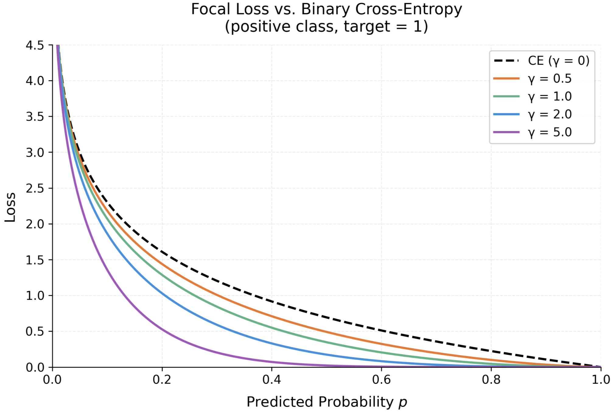
Eq. 2 The formula for alpha-balanced cross-entropy loss²². Lin et al.²² introduced focal loss to mitigate effects of class imbalance, multiplying by a focal factor (1-pt) with a tunable gamma parameter. The focal factor amplifies losses for difficult, misclassified examples and forces the model to focus on them²², demonstrated in Fig. 1.

Eq. 3 The focal loss formula for one sample²².

Eq. 4 The alpha-balanced focal loss formula for one sample, combining both loss function adjustment techniques²².

Experiments Overview

The Ultralytics Python library was used to train a YOLOv12-s model on the NMCD^6,14,16. Several hyperparameters were divided into categories based on their functions and tuned to increase model performance. Tuned values created the final model configuration, evaluated on the test set. Models were evaluated primarily using mAP50 and mAP50-95⁷.

Methods

Dataset

NMCD, the dataset used in this work, contains 10 different object classes to detect and classify, 9 of which are cytotypes. Epithelial cells make up the majority of nasal mucosa. Ciliated and metaplastic cells are epithelial cells that appear tailed and round, respectively. Muciparous cells are associated with more mucus and have a two-part shape. Eosinophils are associated with allergies. Neutrophil cells, which are smaller than eosinophils, signify an immune reaction, are round, and have many nucleoli. Lymphocytes, necessary for immune responses, are surrounded in a ring. Mast cells are large, oval, and associated with present allergies. Emazia cells are red blood cells associated with prior wounds or abnormalities. Artifacts are non-cells that appear similar to cells⁶.

NMCD took data from patients at the Rhinology Clinic of the University of Bari’s Otolaryngology Department. No other demographic or medical information on participants was given by the authors. 14 nasal mucosa slides were collected using a swab, applying the May-Grunwald-Giemsa staining technique for color. 50 pictures were taken of each slide, 700 1024×768 resolution images in total, using a ProWay XSZPW208T microscope set to 1000x zoom with a 3MP DCE-PW300 camera. Experts manually annotated each image with bounding boxes and class labels, and annotation disputes were settled by votes. Low-quality images were dropped, resulting in a final total of 500 images. No slide or patient identifiers were given in the dataset. Two sample images from the training dataset are shown in Fig. 2⁶.

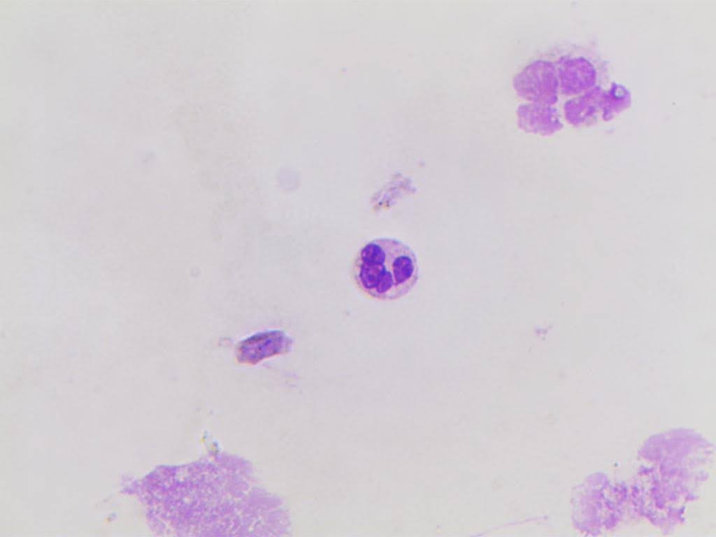
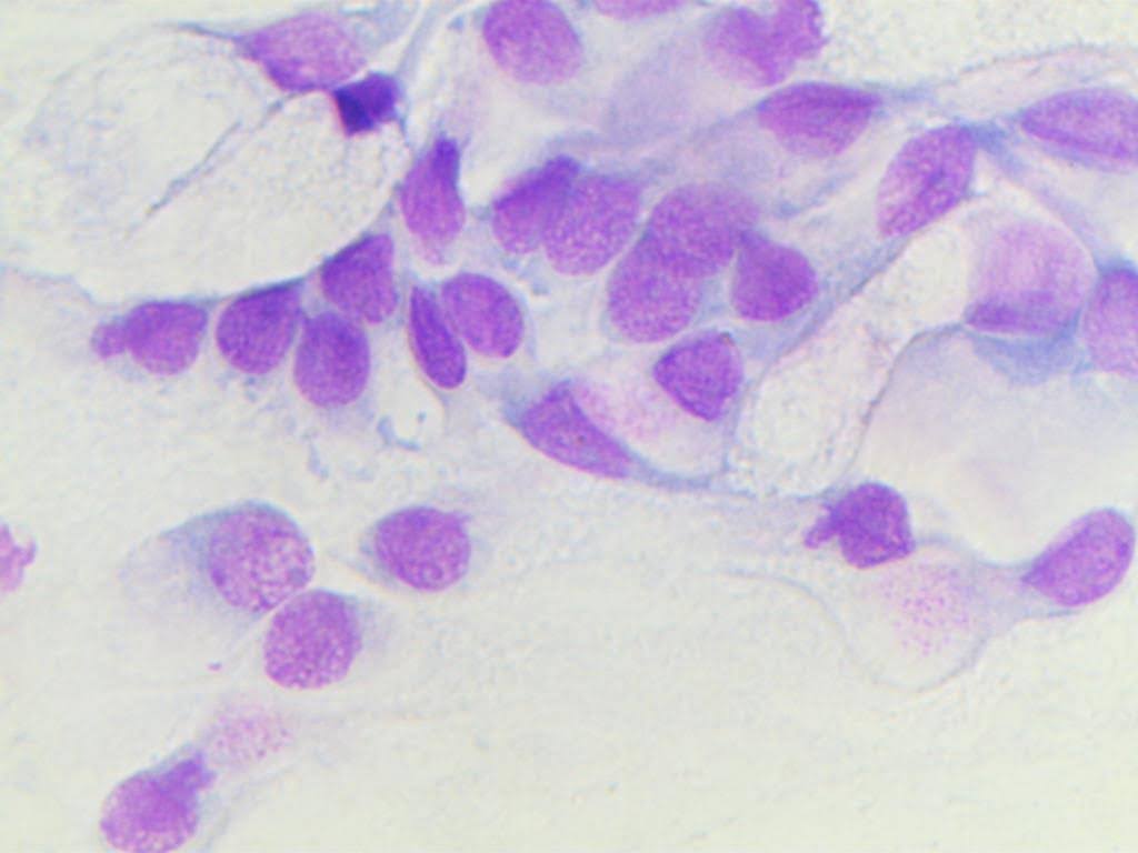
Figure 2 | Example images from the NMCD training dataset⁶.

Hyperparameters Selected

Hyperparameters were divided into 6 categories based on their effects. Basic hyperparameters, which adjusted the model without augmenting data, were selected to replicate commonly adjusted configurations for object detection, as the dataset authors did not disclose their hyperparameter selection⁶: batch size, learning rate, image size, model patience, weight decay²⁴, optimizer, and number of epochs. Some were selected: the AdamW optimizer was used because of its better generalization to new data and faster convergence over Adam²⁴; epochs and patience were kept constant at 600 and 50; and batch size was kept at 16. The rest were tuned.

Data augmentations made up the bulk of the adjusted hyperparameters, spanning 4 categories. The first category of augmentations, spatial transformations, included degrees, translation, and flips. Degrees rotated the original input image in either direction, while translate shifted the image along either axis, by randomly chosen angles in degrees and factors up to the corresponding hyperparameters, respectively. Up-down and left-right flips reflected the original image over the horizontal and vertical axes, respectively, with the probabilities of the corresponding hyperparameters.

Geometric distortions simulated variations in cell morphology and viewpoint: scale, shear, and perspective. Scale shrunk or expanded the image by a randomly selected factor up to the given value, simulating size variation between cells of the same class while preserving internal angles and proportions. Shear rotated the 2 axes by randomly selected amounts in either direction up to shear hyperparameter in degrees, creating a distortion effect. Perspective transformation was applied with a magnitude within [-v, v], where v was the specified value.

Compositional augmentations combined multiple images from the dataset to create a new sample. These included mixup, mosaic, and copy-paste. Mosaic cropped 4 images and placed them next to each other, diversifying the image while keeping the images themselves untouched. Mixup augmentation combined two images by linearly combining their values and labels. Zhang et al.’s²⁵ experiments demonstrated that mixup led to better generalization with new data. Mosaic and mixup were applied with a probability of their respective hyperparameters.

Since Ultralytics did not support its use for object detection, copy-paste augmentation was implemented from scratch and applied to the training dataset before model training. This work’s implementation stored an augmented dataset double the size of the original training set to mimic Ultralytics’ implemented augmentations effective increasing of dataset size by applying different random augmentations throughout training. While typically only done for segmentation, where precise ground truth masks allow for more seamless pasting, it is acceptable in this situation because cell stain backgrounds are dull and featureless.

The total number of crops pasted onto each image was selected from a uniform distribution from 1 to 5, keeping variety without overcrowding. Two methods of copy-paste were employed: rectangular and elliptical alpha blending. If both performed better than the baseline on the validation dataset, only the better-performing one was chosen.

In rectangular copy-paste, pasted instances’ rectangular borders were feathered to smoothly integrate cropped cells’ backgrounds. On the other hand, elliptical alpha blending used the ellipse inscribed in the pasted instance’s rectangle as a mask. The inner 85%, determined by normalized distance to the center of the mask, was purely the pasted instance, while the outer 15% was a weighted blend of the foreground (pasted instance) and background (original image). Regions outside the elliptical mask were kept as the original image. Elliptical alpha blending effectively served as a makeshift segmentation mask, better representing cell shape, when such masks were not available.

Fig. 3 demonstrates the noticeable difference between the two approaches. In Fig. 3a., large portions of the pasted instances’ background are shown, disrupting the image and making it look unnatural and obviously pasted. In Fig. 3b, the elliptical masks fit the cell shape well, smoothly integrating the pasted instances into the image.

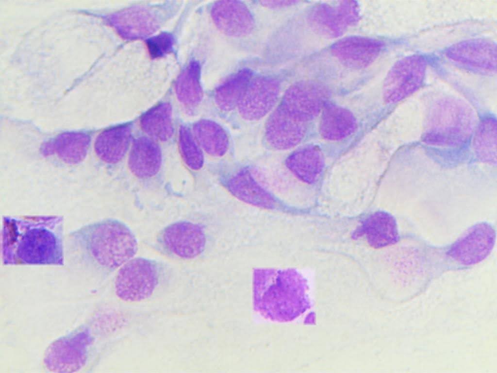
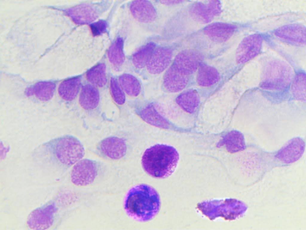
Figure 3 | a) training image with rectangular copy-paste. b) training image with elliptical alpha blending copy-paste.

The class of each paste was chosen randomly from the probability distribution given by the inverse (reciprocal) of the training set cytotype distribution raised to a tuned exponent δ (lowercase delta) for rectangular pasting, ψ (lowercase phi) for elliptical alpha blended pasting, and normalized to sum to 1.

Eq. 5 The formula for the probability p_i that the pasted instance belongs to class i, where n_c is the number of instances of class c, and C is the set of all classes in the dataset.

Photometric transformations adjusted lighting and texture: hue, saturation, and value (HSV), blur, and togray augmentations. HSV augmentations varied the color of the input images, making the model more robust to environment and cell stain lighting variation. Hue, saturation, and value changed color wheel position, color intensity, and brightness, respectively, by a fraction up to the corresponding hyperparameters.

Blur passes a Gaussian distribution kernel across the image, similarly to a convolutional kernel. Gaussian blurring removes fine, noisy details that can hurt model performance and forces the model to focus on larger features²⁶. Togray applied a grayscale transformation to the input image with a probability of the togray hyperparameter, forcing the model to focus more on cell morphology and less on lighting. Blur and togray were applied with probabilities of their respective hyperparameters.

Eq. 6 The formula for the Gaussian blur kernel f(x, y) at pixel (x, y), where A is the amplitude of the function, (x₀, y₀) is the center of the kernel, and σ_x and σ_y are the kernel’s standard deviations on the x and y axes, respectively²⁶.

Finally, loss function hyperparameters, namely the α vector and γ²², adjusted the loss function formula discussed in the loss functions section. Similarly to copy-paste, alpha weights were obtained from a normalized inverse training dataset class distribution exponentiated with a tunable exponent β, shown in Eq. 7. This implementation assigned greater importance to minor classes while decreasing the search space for the alpha vector to only one hyperparameter.

Eq. 7 The formula for alpha weight i for every class i, where ni is the number of instances of the i’th class, and C is the set of all classes in the dataset.

Model Development and Testing

The model was developed by tuning numerous hyperparameters with various effects, selecting ideal configurations based on validation mAP50-95. Due to Google Colab’s usage limits, validating configurations was done on three training runs each. All trials that informed model development choices used only the validation dataset for evaluating model performance.

Ultralytics version 8.4.21 was used¹⁴ and Colab’s 2026.04 runtime version was selected. Uncontrollable variation in CUDA versions on Colab runtimes may lead to small discrepancies when reproducing this work’s experiments. Trials were mainly run using the A100 GPU, taking approximately 12 minutes on average. The small size of the YOLOv12 model was used because of Google Colab’s usage limits; furthermore, using larger versions of the same architecture is expected to yield better results with diminishing returns, as demonstrated in the YOLOv12 paper with YOLOv12 on the COCO dataset^16,17.

Hyperparameters were tuned individually by running ablation trials over multiple candidate values and finding the optimal one. During ablations, basic hyperparameters were not adjusted from the replicated baseline values. Individual hyperparameter ablating was evaluated with mAP50, which played no role in model selection, and mAP50-95⁷. Candidate values were trained and evaluated on 3 random seeds each, then the mAP50-95 values were bootstrapped 1000 times to obtain the value’s reported mean mAP50-95. Non-default values were adopted only if their reported mean mAP50-95 exceeded that of the default by at least the sample standard deviation of the value’s 3 mAP50-95’s. If more than one hyperparameter value outperformed the baseline by at least a standard deviation, the value with the higher bootstrapped mAP50-95 mean was adopted.

First, initial and final learning rate and weight decay were tuned, while keeping the rest of the 3 at their default values and comparing to the nontuned basic hyperparameter configuration. Second, the baseline configuration, created from both the selected and tuned basic hyperparameter values, was evaluated on the validation set on 3 random seeds with mAP50 and mAP50-95. Then, non-basic hyperparameters were tuned by comparing to the baseline.

Finally, the baseline and final models were tested. The final model was configured by using the basic hyperparameter configuration and all chosen hyperparameter values from ablation experiments. Performance was measured with per-class box-precision, box-recall, and  F1 score at IoU threshold 0.5, as well as AP50, AP50-95, averages of those metrics, precision-recall curves, and confusion matrices. Baseline and final model configurations were evaluated by training and testing using 5 random seeds each.

Performance metrics

All metrics, graphs, and confusion matrices were measured and created by Ultralytics¹⁴. 5 metrics were used in model evaluation: box-precision, box-recall, F1 score, mAP50, and mAP50-95. The primary model performance metrics are mAP50-95, as specified in the COCO detection evaluation protocol, as well as mAP50⁷.

Intersection over union (IoU) quantifies how much the predicted box matches the ground truth box, shown in Eq. 8. IoU thresholds determine at what IoU a prediction is considered to match ground truth boxes. Box-precision, written in Eq. 9, measures the portion of predicted boxes that are true positives, overlapping with a ground truth positive with an IoU of at least the IoU threshold. Box-recall, shown in Eq. 10, measures the portion of ground truth instances that the model predicted a bounding box for with IoU of at least the IoU threshold. Average precision (AP), shown in Eq. 11, combines both box-precision and box-recall into one number for 1 class by calculating the area under the precision-recall curve over all confidence thresholds⁷.

Eq. 8 Formula for IoU, where A and B represent the two rectangles being evaluated⁷.

Eq. 9 Box-precision formula, where TP is the number of true positives, and FP is the number of false positives⁷.

Eq. 10 Box-recall formula, where TP is the number of true positives, and FN is the number of false negatives⁷.

Eq. 11 Average box-precision formula, where r and prec(r) are the box-recall and box-precision given the box-recall, respectively, at the specified IoU threshold⁷. Ultralytics calculates AP using interpolation with 101 evenly-spaced recall values between 0 and 1 to make the precision-recall graph decreasing and thus smoother¹⁴.

Mean average precision (mAP) measures performance of all classes, taking the arithmetic mean of each class’s AP. mAP50 only uses an IoU threshold of 50%. On the other hand, mAP50-95 considers IoU thresholds multiples of 5% from 50% to 95% inclusive. Thus, mAP50 is more lenient on localization errors, while mAP50-95 is less forgiving⁷.

Baseline and final model metrics were reported using mean ± sample standard deviation and were measured from the same configuration using different random seeds. Given the exploratory nature of this study, no statistical tests were performed, thus no p values, statistical significance scores, or confidence intervals were reported.

Ethical considerations

Other than using the nasal mucosa dataset, this model did not use any data that could create privacy concerns. Due to the lack of clinical trials, expert validation, and accuracy, the model is not ready to be used in a clinical setting.

Results

Ablation Experiments

Individual hyperparameter ablation validation set results are discussed below. Bold indicates the selected hyperparameter value, and default values were marked with (default). The reported mAP50-95 values are the bootstrapped means described in the Model Development and Testing section, and the reported mAP50 values are calculated in a similar way.

1a. Degrees	mAP50	mAP50-95	1b. Translate	mAP50	mAP50-95
0 (default)	0.449	0.240	0	0.438	0.234
90	0.474	0.258	0.1 (default)	0.449	0.240
180	0.497	0.272	0.2	0.455	0.247
			0.3	0.491	0.27
			0.4	0.464	0.25
1c. Flip (LR)	mAP50	mAP50-95	1d. Flip (UD)	mAP50	mAP50-95
0	0.434	0.233	0 (default)	0.449	0.240
0.5 (default)	0.449	0.240	0.5	0.507	0.272

As shown in Table 1a, 180 was selected as the value for the degrees hyperparameter, assigning a uniformly random rotational angle to each image and simulating camera and cell variations. Table 1b shows that 0.3 was optimal for translation, optimizing its tradeoff between increased robustness from spatial adjustment and loss of data from part of the image leaving the screen. Cell handedness on either axis was shown to be irrelevant, as both axes’ flips at 0.5 probability benefitted model performance, demonstrated in Table 1c and 1d.

2a. Scale	mAP50	mAP50-95	2b. Shear	mAP50	mAP50-95
0.3	0.445	0.236	0.0 (default)	0.449	0.240
0.5 (default)	0.449	0.240	0.5	0.452	0.242
0.7	0.45	0.239	1.0	0.461	0.246
			5.0	0.458	0.235
2c. Perspective	mAP50	mAP50-95
0 (default)	0.449	0.240
1e-5	0.453	0.245
1e-4	0.479	0.256

As shown in Table 2a, 0.5 was found to be the optimal scaling hyperparameter. Table 2b and Table 2c show that, despite both shear and perspective deforming internal cell structure, shear applied in small amounts did not exceed baseline performance by at least a standard deviation, while perspective effectively simulated data camera angle diversity and increased model performance by more than a standard deviation.

3a. Mosaic	mAP50	mAP50-95	3b. Mixup	mAP50	mAP50-95
0.6	0.456	0.241	0.0 (default)	0.449	0.240
0.8	0.444	0.239	0.01	0.427	0.227
1.0 (default)	0.449	0.240	0.02	0.461	0.244
3c. Delta (rectangular copy-paste exponent)	mAP50	mAP50-95	3d. Phi(elliptical alpha blended copy-paste exponent)	mAP50	mAP50-95
No copy-paste (default)	0.449	0.240	No copy-paste (default)	0.449	0.240
0.0	0.447	0.24	0.0	0.482	0.255
1.0	0.478	0.256	1.0	0.469	0.248
2.0	0.464	0.247	2.0	0.478	0.254

Table 3a and Table 3b show that neither mosaic nor mixup had a clear performance trend, and both were kept at the default values. Table 3c and Table 3d show that both copy-paste methods improved performance over the baseline by more than a standard deviation; however, only rectangular copy-paste was adopted since it outperformed elliptical alpha blended copy-paste.

4a. hsv_h	mAP50	mAP50-95	4b. hsv_s	mAP50	mAP50-95
0.005	0.44	0.24	0.5	0.471	0.25
0.015 (default)	0.449	0.240	0.7 (default)	0.449	0.240
0.025	0.479	0.26	0.9	0.448	0.239
4c. hsv_v	mAP50	mAP50-95	4d. blur	mAP50	mAP50-95
0.2	0.478	0.259	0.01 (default)	0.449	0.240
0.4 (default)	0.449	0.240	0.1	0.466	0.25
0.6	0.45	0.242	0.2	0.463	0.255
4e. togray	mAP50	mAP50-95
0.01 (default)	0.449	0.240
0.1	0.456	0.245
0.2	0.465	0.263

Table 4c shows that applying weaker value augmentation increased performance by over a standard deviation, suggesting that cell brightness may be important to cell classification. Table 4a and Table 4b show that the non-default hue and saturation augmentation values did not exceed baseline performance by at least a standard deviation. Table 4d and Table 4e show that the optimal blur and togray probabilities were both 0.2. Blurring and grayscaling force the model to focus on only color and only morphology, respectively, and may increase performance by allowing it to focus on only one of these two aspects at a time during training.

5a. Beta	mAP50	mAP50-95	5b. Gamma	mAP50	mAP50-95
0 (default)	0.447	0.240	0 (default)	0.447	0.240
0.5	0.451	0.247	0.5	0.467	0.248
1.0	0.407	0.219	1.0	0.453	0.242

Table 5a demonstrates that alpha balancing, even in small amounts, did not help address model performance deficiency caused by class imbalance enough to boost performance by at least a standard deviation. Table 5b shows that focal loss with a mild value of 0.5 increased mAP50 and mAP50-95 by more than a standard deviation.

Model Testing

The replicated baseline model configuration, which used YOLOv12-s, achieved an mAP50 of 0.482 ± 0.021 and an mAP50-95 of 0.283 ± 0.012. As shown in Table 6 and Fig. 4a, the 3 classes with the highest AP50-95 were the 3 majority classes, eosinophil, epithelial, and neutrophil, which may be attributed to the dataset providing more information on those classes to the model during training. Mast cell box-precision was 1.000 and box-recall was 0.000, meaning that the model did not classify any objects as mast cells, likely because it did not learn enough about the class.

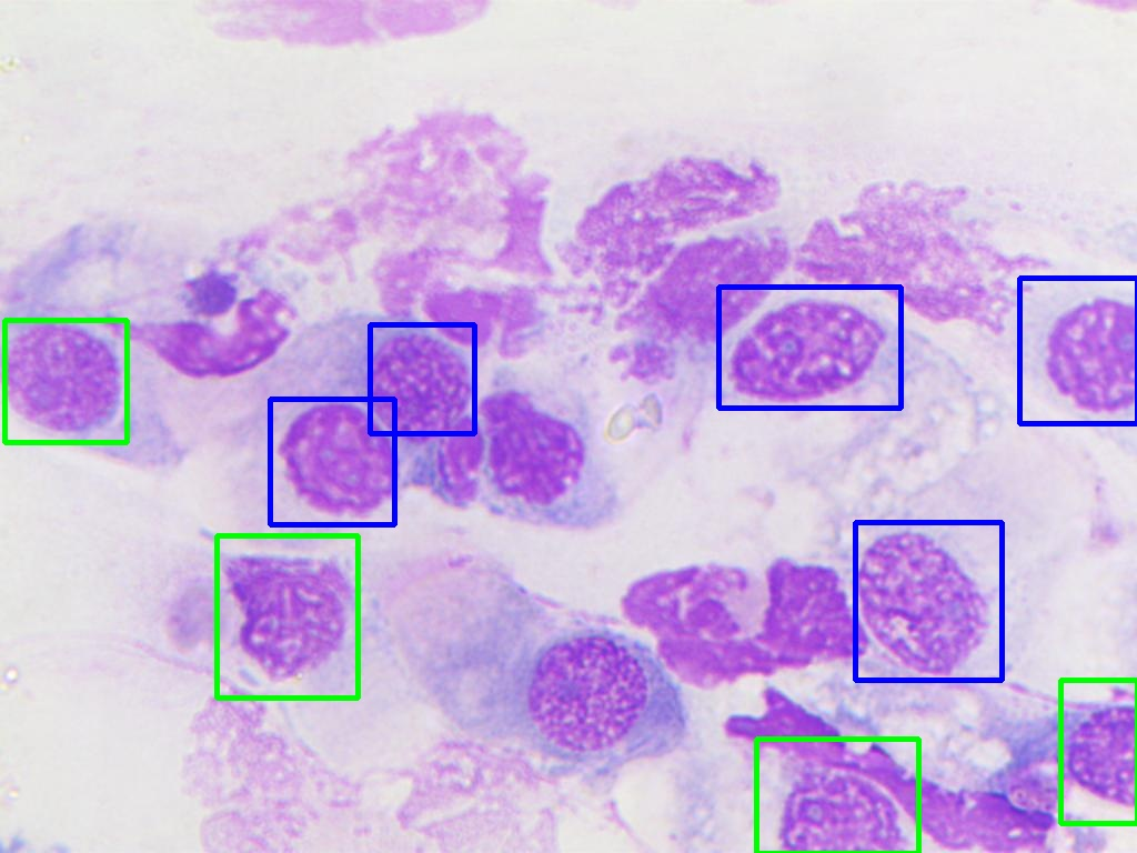
However, the 4 minority classes, defined as those with less than 100 training instances, bolded in Table 6 were not strictly the lowest performing ones. Artifact, metaplastic, and muciparous all scored lower AP50-95 than epithelial ciliated, a minority class, demonstrating that the number of cells in the training set for each class may not be the only major factor in performance on the test set. Another potential factor is that some classes are more similar to other classes, making them harder to distinguish, while others are more distinctive. For example, epithelial and metaplastic cells belong to the overarching epithelial cell class and thus are more similar in appearance, as shown in Fig. 6⁶. This idea is also shown by eosinophil scoring over double the AP50-95 of muciparous cells despite only having 17 more training instances⁶.

Fig. 5a shows that most of the errors, represented by off-diagonal entries, are on the borders, which represent confusing artifacts with cells, or objects with background, not misclassifying a cell as another type of cell. A majority of the interior of the matrix was empty, indicating no confusion between most pairs of cell classes.

The final model configuration scored 0.552 ± 0.019 mAP50 and 0.321 ± 0.010 mAP50-95, corresponding to moderate increases of 14.5% and 13.4% relative to the baseline, respectively. Improvement in AP50-95 was observed for all classes except for two of the minority classes, epithelial ciliated and mast cell, shown in Table 7. Epithelial ciliated AP50-95 decreased by 1.8%, and mast cell box-precision decreased by 80% while box-recall remained 0, demonstrating that the final model was confident enough to wrongly classify some objects as mast cells, although it made no such correct predictions.

The decrease in performance of these two classes was likely due to the class-imbalance techniques applied: copy-paste and focal loss potentially allowed the model to overfit to the training dataset by focusing on and repeating the same few instances several times. While data augmentations can increase training data diversity, the amount of data for the minority classes in the NMCD may have been too small⁶ to provide the model with enough relevant signal. Similarly, the increase in majority cell class performance may have been because such classes had enough training data for the model to learn.

However, despite having only 37 training set instances, less than epithelial ciliated⁶, emazia AP50-95 substantially increased by 119.1%, and metaplastic cell AP50-95 remained at a low 0.080, despite having 184 training instances⁶, suggesting that class imbalance is not the only major factor for performance effects of hyperparameter adjustments, and that other factors may also play a role, such as the previously discussed varying amount of distinction between classes. However, the general trend in per-class model performance remains: minority classes have lower baseline performance compared to majority classes and are more likely to perform worse after augmentations and class imbalance techniques.

Fig. 4b shows that the emazia performance in the median-performing model was notably higher than that of each of the 3 majority classes, which are higher than in Fig. 4a. Fig. 5b shows that the amount of false negatives when distinguishing cells from background notably increased by 83.1%, from 236 to 432, demonstrating that the data augmentations, while allowing the model to more precisely distinguish different cytotypes by training on data with more variety, may have impaired the model’s ability to distinguish foreground from background.

Class	Box-P	Box-R	Box-F1	AP50	AP50-95
artifact	0.420±0.048	0.416±0.030	0.415±0.012	0.363±0.033	0.220±0.025
emazia	0.790±0.348	0.144±0.167	0.208±0.243	0.385±0.286	0.230±0.184
eosinophil	0.722±0.043	0.835±0.016	0.774±0.030	0.819±0.020	0.494±0.016
epithelial	0.693±0.045	0.924±0.021	0.791±0.023	0.869±0.011	0.508±0.009
epithelial ciliated	0.471±0.167	0.564±0.149	0.495±0.103	0.531±0.121	0.382±0.087
lymphocyte	0.481±0.234	0.175±0.046	0.235±0.037	0.274±0.049	0.165±0.042
mast cell	1.000±0.000	0.000±0.000	0.000±0.000	0.071±0.105	0.055±0.085
metaplastic	0.203±0.069	0.276±0.040	0.231±0.058	0.137±0.039	0.079±0.028
muciparous	0.597±0.078	0.469±0.063	0.518±0.014	0.534±0.042	0.240±0.036
neutrophil	0.668±0.047	0.848±0.026	0.746±0.023	0.839±0.008	0.456±0.005
average	0.604±0.083	0.465±0.024	0.441±0.011	0.482±0.021	0.283±0.012

Class	Box-P	Box-R	Box-F1	AP50	AP50-95
artifact	0.430±0.019 ↑	0.448±0.073 ↑	0.435±0.025 ↑	0.412±0.036 ↑	0.245±0.019 ↑
emazia	0.840±0.133 ↑	0.760±0.249 ↑	0.784±0.172 ↑	0.908±0.107 ↑	0.504±0.031 ↑
eosinophil	0.759±0.049 ↑	0.885±0.036 ↑	0.816±0.028 ↑	0.881±0.020 ↑	0.540±0.026 ↑
epithelial	0.697±0.048 ↑	0.915±0.028 ↓	0.790±0.024 ↓	0.881±0.010 ↑	0.511±0.009 ↑
epithelial ciliated	0.379±0.092 ↓	0.571±0.161 ↑	0.437±0.065 ↓	0.515±0.175 ↓	0.375±0.124 ↓
lymphocyte	0.467±0.305 ↓	0.282±0.188 ↑	0.262±0.153 ↑	0.355±0.052 ↑	0.208±0.036 ↑
mast cell	0.200±0.447 ↓	0.000±0.000	0.000±0.000	0.039±0.033 ↓	0.026±0.026 ↓
metaplastic	0.177±0.056 ↓	0.226±0.137 ↓	0.186±0.079 ↓	0.147±0.031 ↑	0.080±0.013 ↑
muciparous	0.651±0.118 ↑	0.444±0.132 ↓	0.505±0.080 ↓	0.533±0.033 ↓	0.245±0.009 ↑
neutrophil	0.739±0.041 ↑	0.845±0.018 ↑	0.787±0.018 ↑	0.852±0.006 ↑	0.477±0.013 ↑
average	0.534±0.075 ↓	0.538±0.040 ↑	0.500±0.038 ↑	0.552±0.019 ↑	0.321±0.010 ↑

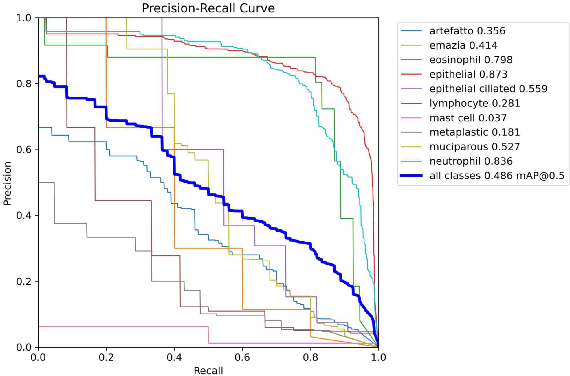
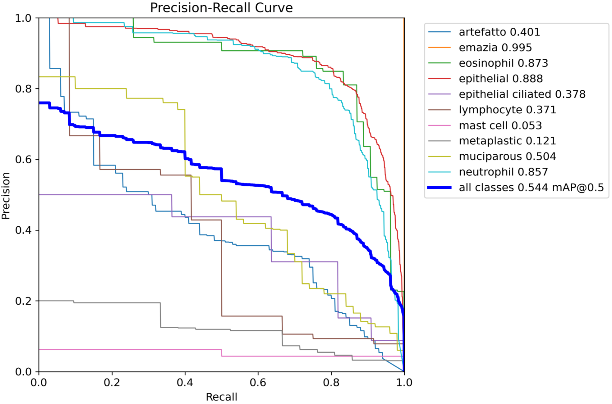
Figure 4 | a: precision-recall curve of median-performing baseline model. b: precision-recall curve of median-performing final model. Median-performing models were chosen using mAP50-95 alone.

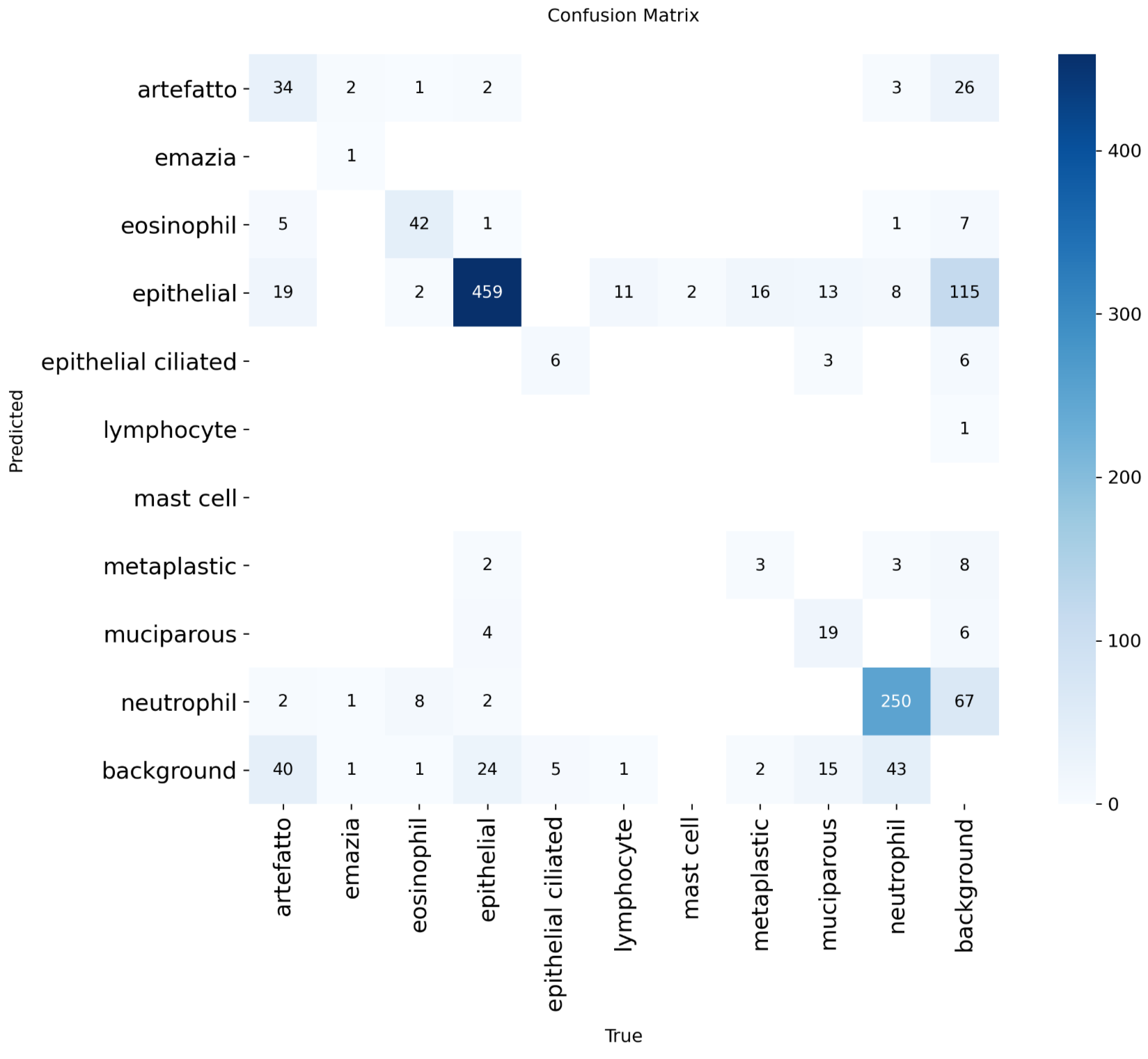
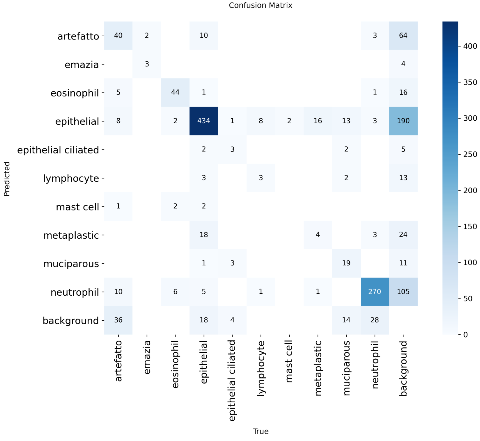
Figure 5 | a: confusion matrix of median-performing baseline model. b: confusion matrix of median-performing final model. Median-performing models were chosen using mAP50-95 alone.

Discussion

This work’s highest-performing model achieved mAP50 0.552 ± 0.019 and mAP50-95 0.321 ± 0.010 on the test set. This represents moderate improvements of 0.070 (+14.5%) in mAP50 and 0.038 (+13.4%) in mAP50-95 compared to the baseline model. Hyperparameter tuning for the object detection in nasal cytology task yielded modest improvements in model performance. Thus, both objectives of improving model performance and evaluating hyperparameter effects were met.

Alpha balancing did not improve model performance, potentially because it reweighted cell instances’ importance while only considering class imbalance, using a rigid constant multipler and ignoring other potential factors that may determine difficulty of predicting. On the other hand, focal loss is more adaptive to errors, as it reweighted cell instances’ importance by the incorrectness of predictions. This approach directly found the model’s errors and areas to improve.

Elliptical alpha blended copy-paste was a technique implemented from scratch rather than using an existing framework, designed for the nasal mucosa detection and classification task specifically. However, elliptical alpha blending may have not always captured cell borders accurately, leaving parts of them out, and borders are distinct features of cell classes. For example, muciparous cells have a chromatin reinforced membrane⁶. This may have led to underperformance when compared to rectangular copy-paste. In contrast, while rectangular copy-paste incorporated pasted instances inaccurately and created choppy borders in the background, it captured the whole cell border, assuming the ground truth labels were correct.

Although QANIC achieved higher performance, its classification model only learned how to distinguish between 2 of the most common cytotypes, grouping all other cells into a miscellaneous category⁴. Additional research in this task is necessary to produce a sufficiently high-performing model for clinical implementation. A similar work compared the efficacy of several YOLO architectures in detecting and classifying pressure ulcers into 4 stages, achieving 0.964 mAP50 and 0.68 mAP50-95 with YOLOv7. Their model was deployed in the form of a mobile app at the Eulji University Medical Center, expediting patient ulcer classification and having 87% accuracy, suggesting that, for clinical implementation, future work should aim for a similar level of performance²⁷. However, object detection in nasal mucosa stain images has more classes and more object density, meaning it may be more complex and difficult to reach similar results.

The major limitations were Google Colab’s usage limits and the dataset’s class imbalance and small size. Statistical testing was not performed because of the exploratory nature of the work. The amount of seeds needed to produce sufficiently narrow confidence intervals for demonstrating outperformance would be outside the computational budget.

The NMCD has only 14 slides, meaning a maximum of 14 patients, thus the model could have learned noisy cell characteristics of those specific patients. The dataset’s reliance on a single rhinology clinic reduced data diversity and could further limit model generalizability when deployed to various populations⁶. Extensively tuning hyperparameters may have overfit to the validation dataset and harmed test results. Hyperparameter ablation performance was only measured with mAP50 and mAP50-95, thus only the general performance trends were tracked.

The hyperparameter selection method used did not consider interactions between hyperparameters that can play a role in model performance, and taking such interactions into account when optimizing may boost performance. Alternative approaches, including Bayesian optimization and evolutionary search, were not utilized since they would not have helped characterize the individual effects of the hyperparameters on model performance. Additionally, the massive amount of trials needed to optimize using Bayesian optimization in a high dimensional search space or using evolutionary algorithms was outside of the computational budget.

Additionally, due to the lack of slide and patient identifiers in the dataset, using a grouped validation approach in the model selection process to keep each slide in only one data split could not be done. Thus, the model may have learned features of the slide itself such as slide-specific cellularity, patient-specific cell characteristics, and lighting. Ultimately, the numbers presented are optimistic since this form of data leakage may have artificially boosted performance.

Future recommendations for fundamental changes to further enhance model performance include utilizing object detection architectures that may be released after this paper, as well as YOLO26¹⁴, the latest iteration of YOLO. Using a larger model size or creating a specialized architecture for nasal mucosa cell detection rather than choosing a hyperparameter configuration alone may also yield superior results. Training procedures designed for situations with imbalanced or small datasets may also be beneficial to performance; for example, semi-supervised learning, in which the model can be trained on unlabeled data when it makes confident predictions, and human experts annotate the unlabeled data that the model makes the most unconfident predictions on, essentially allowing human expertise to guide the model. Another example is transfer learning; a model could be trained on large microscope cell image datasets from various cytology subfields before being trained on nasal mucosa-specific data.

Another recommendation is obtaining or synthetically generating more data from various populations, as the small dataset did not provide enough information for the model to learn meaningful signal on certain classes, as suggested by the experiments. Labeling data with patient diagnoses would also provide meaningful context. 

Once model performance is sufficiently improved, future work should also obtain clinical validation to drive object-detection-powered nasal cytology with several classes towards clinical application. Clinically validating the usefulness of a model for diagnosis would require the aforementioned patient labels, as well as model performance optimization for cellularity accuracy specifically, such as lowering the per-slide, per-class cell count mean absolute error. 

In conclusion, tuning data augmentation and loss function hyperparameters, as well as applying rectangular copy-paste, led to moderate improvements in mAP50 and mAP50-95 on the nasal mucosa cell detection and classification task. Additional research implementing a specialized architecture and training method, collecting more data, leveraging larger models, and addressing limitations in this work may further improve model performance to be sufficiently robust for clinical validation and implementation.

Acknowledgments

I would like to thank my mentor Anthony Cuturrufo, a PhD student at UCLA, for his tremendous help with this paper. I would also like to thank Inspirit AI for their assistance.

References

1. G. Paoletti, L. Malvezzi, A. M. Riccio, D. Descalzi, F. Pirola, E. Russo, L. De Ferrari, F. Racca, S. Ferri, M. R. Messina, F. Puggioni, E. Nappi, D. Bagnasco, F. R. Canevari, F. Grizzi, G. Mercante, G. Spriano, G. W. Canonica, E. Heffler. Nasal cytology as a reliable non-invasive procedure to phenotype patients with type 2 chronic rhinosinusitis with nasal polyps. World Allergy Organization Journal. Vol. 15, pg. 100700, 2022 https://doi.org/10.1016/j.waojou.2022.100700 [↩] [↩]
2. M. A. Al-Abbadi. Basics of cytology. Avicenna Journal of Medicine. Vol. 1, pg. 18–28, 2011 https://doi.org/10.4103/2231-0770.83719 [↩]
3. M. S. Landau, L. Pantanowitz. Artificial intelligence in cytopathology: a review of the literature and overview of commercial landscape. Journal of the American Society of Cytopathology. Vol. 8, pg. 230–241, 2019 https://doi.org/10.1016/j.jasc.2019.03.003 [↩]
4. X. Zhang, X. Xu, W. Liu, L. Qin, Y. Song, J. Li, L. Xi, C. Wang, L. Zhang, Y. Zhang. Development of artificial intelligence for quantitative assessment of nasal inflammatory cytology in chronic rhinitis by whole-slide images. International Forum of Allergy & Rhinology. Vol. 16, pg. 272–282, 2026 https://doi.org/10.1002/alr.70075 [↩] [↩] [↩]
5. M. Yaseen. What is yolov8: an in-depth exploration of the internal features of the next-generation object detector. Preprint at https://arxiv.org/abs/2408.15857 2024 https://doi.org/10.48550/ARXIV.2408.15857 [↩]
6. M. G. Camporeale, G. Dimauro, M. Gelardi, G. Iacobellis, M. S. Ladisa, S. Latrofa, N. Lomonte. A nasal cytology dataset for object detection and deep learning. Biomedical Signal Processing and Control. Vol. 114, pg. 109263, 2026 https://doi.org/10.1016/j.bspc.2025.109263 [↩] [↩] [↩] [↩] [↩] [↩] [↩] [↩] [↩] [↩] [↩] [↩] [↩] [↩] [↩] [↩]
7. R. Padilla, W. L. Passos, T. L. B. Dias, S. L. Netto, E. A. B. da Silva. A comparative analysis of object detection metrics with a companion open-source toolkit. Electronics. Vol. 10, 2021 https://doi.org/10.3390/electronics10030279 [↩] [↩] [↩] [↩] [↩] [↩] [↩] [↩] [↩] [↩]
8. A. Esteva, K. Chou, S. Yeung, N. Naik, A. Madani, A. Mottaghi, Y. Liu, E. Topol, J. Dean, R. Socher. Deep learning-enabled medical computer vision. Npj Digital Medicine. Vol. 4, pg. 5, 2021 https://doi.org/10.1038/s41746-020-00376-2 [↩]
9. O. Ronneberger, P. Fischer, T. Brox. U-net: convolutional networks for biomedical image segmentation. in Medical Image Computing and Computer-Assisted Intervention – MICCAI 2015 (eds N. Navab, J. Hornegger, W. M. Wells & A. F. Frangi) pg. 234–241, Springer International Publishing, Cham, 2015 https://doi.org/10.1007/978-3-319-24574-4_28 [↩] [↩]
10. A. Archit, L. Freckmann, S. Nair, N. Khalid, P. Hilt, V. Rajashekar, M. Freitag, C. Teuber, M. Spitzner, C. Tapia Contreras, G. Buckley, S. von Haaren, S. Gupta, M. Grade, M. Wirth, G. Schneider, A. Dengel, S. Ahmed, C. Pape. Segment anything for microscopy. Nature Methods. Vol. 22, pg. 579–591, 2025 https://doi.org/10.1038/s41592-024-02580-4 [↩] [↩]
11. A. Kirillov, E. Mintun, N. Ravi, H. Mao, C. Rolland, L. Gustafson, T. Xiao, S. Whitehead, A. C. Berg, W.-Y. Lo, P. Dollár, R. Girshick. Segment anything. in 2023 IEEE/CVF International Conference on Computer Vision (ICCV) pg. 3992–4003, 2023 https://doi.org/10.1109/ICCV51070.2023.00371 [↩]
12. Z.-Q. Zhao, P. Zheng, S.-T. Xu, X. Wu. Object detection with deep learning: a review. IEEE Transactions on Neural Networks and Learning Systems. Vol. 30, pg. 3212–3232, 2019 https://doi.org/10.1109/TNNLS.2018.2876865 [↩]
13. M. G. Ragab, S. J. Abdulkadir, A. Muneer, A. Alqushaibi, E. H. Sumiea, R. Qureshi, S. M. Al-Selwi, H. Alhussian. A comprehensive systematic review of yolo for medical object detection (2018 to 2023). IEEE Access. Vol. 12, pg. 57815–57836, 2024 https://doi.org/10.1109/ACCESS.2024.3386826 [↩] [↩]
14. G. Jocher, J. Qiu, M. Liu, S. Lyu, F. C. Akyon, M. E. Kalfaoglu. Ultralytics yolo26: unified real-time end-to-end vision models. Preprint at https://arxiv.org/abs/2606.03748 2026 https://doi.org/10.48550/arXiv.2606.03748 [↩] [↩] [↩] [↩] [↩] [↩]
15. A. Vaswani, N. Shazeer, N. Parmar, J. Uszkoreit, L. Jones, A. N. Gomez, L. Kaiser, I. Polosukhin. Attention is all you need. in Advances in Neural Information Processing Systems (eds I. Guyon, U. V. Luxburg, S. Bengio, H. Wallach, R. Fergus, S. Vishwanathan & R. Garnett) Vol. 30 Curran Associates, Inc., 2017 [↩]
16. Y. Tian, Q. Ye, D. DOERMANN. YOLOv12: attention-centric real-time object detectors. in Advances in Neural Information Processing Systems (eds D. Belgrave, C. Zhang, H. Lin, R. Pascanu, P. Koniusz, M. Ghassemi & N. Chen) Vol. 38, Main Conference pg. 78433–78457, Curran Associates, Inc., 2025 https://doi.org/10.52202/085713-2627 [↩] [↩] [↩] [↩]
17. T.-Y. Lin, M. Maire, S. Belongie, J. Hays, P. Perona, D. Ramanan, P. Dollár, C. L. Zitnick. Microsoft coco: common objects in context. in Computer Vision – ECCV 2014 (eds D. Fleet, T. Pajdla, B. Schiele & T. Tuytelaars) pg. 740–755, Springer International Publishing, Cham, 2014 [↩] [↩]
18. A. Wang, H. Chen, L. Liu, K. Chen, Z. Lin, J. Han, G. Ding. YOLOv10: real-time end-to-end object detection. in Advances in Neural Information Processing Systems (eds A. Globerson, L. Mackey, D. Belgrave, A. Fan, U. Paquet, J. Tomczak & C. Zhang) Vol. 37 pg. 107984–108011, Curran Associates, Inc., 2024 https://doi.org/10.52202/079017-3429 [↩]
19. M. F. Safdar, S. S. Alkobaisi, F. T. Zahra. A comparative analysis of data augmentation approaches for magnetic resonance imaging (mri) scan images of brain tumor. Acta Informatica Medica : AIM : Journal of the Society for Medical Informatics of Bosnia & Herzegovina : Casopis Drustva Za Medicinsku Informatiku BiH. Vol. 28, pg. 29–36, 2020 https://doi.org/10.5455/aim.2020.28.29-36 [↩]
20. Y.-F. Chen, Z.-J. Chen, Y.-Y. Lin, Z.-Q. Lin, C.-N. Chen, M.-L. Yang, J.-Y. Zhang, Y.-Z. Li, Y. Wang, Y.-H. Huang. Stroke risk study based on deep learning-based magnetic resonance imaging carotid plaque automatic segmentation algorithm. Frontiers in Cardiovascular Medicine. Vol. 10, pg. 1101765, 2023 https://doi.org/10.3389/fcvm.2023.1101765 [↩]
21. L. Li, M. Doroslovacki, M. H. Loew. Approximating the gradient of cross-entropy loss function. IEEE Access. Vol. 8, pg. 111626–111635, 2020 https://doi.org/10.1109/ACCESS.2020.3001531 [↩] [↩] [↩]
22. T.-Y. Lin, P. Goyal, R. Girshick, K. He, P. Dollar. Focal loss for dense object detection. in 2017 IEEE International Conference on Computer Vision (ICCV) pg. 2999–3007, IEEE, Venice, 2017 https://doi.org/10.1109/ICCV.2017.324 [↩] [↩] [↩] [↩] [↩] [↩] [↩] [↩]
23. C. Feng, Y. Zhong, Y. Gao, M. R. Scott, W. Huang. TOOD: task-aligned one-stage object detection. in 2021 IEEE/CVF International Conference on Computer Vision (ICCV) pg. 3490–3499, IEEE, Montreal, QC, Canada, 2021 https://doi.org/10.1109/ICCV48922.2021.00349 [↩]
24. I. Loshchilov, F. Hutter. Decoupled weight decay regularization. in International Conference on Learning Representations 2019 [↩] [↩]
25. H. Zhang, M. Cisse, Y. N. Dauphin, D. Lopez-Paz. Mixup: beyond empirical risk minimization. in International Conference on Learning Representations 2018 [↩]
26. E. S. Gedraite, M. Hadad. Investigation on the effect of a gaussian blur in image filtering and segmentation. in Proceedings ELMAR-2011 pg. 393–396, 2011 [↩] [↩]
27. S. H. Jang, C. Ihm, J.-W. Choi, D.-H. Han, K. Bae, M. Kang. Clinical validation of object detection models for ai-based pressure injury stage classification. Diagnostics (Basel, Switzerland). Vol. 16, 2026 https://doi.org/10.3390/diagnostics16050747 [↩]