AI-Driven Forecasting: Deep Learning-Based Predictive Modeling of Wind Power Output to Optimize Clean Energy Supply

Abstract

As global warming poses an imminent threat to human health, renewable energy is even more crucial to combat climate change. Wind energy is one of the cleanest yet cheapest energy sources. However, it generates only 10% of the U.S.’ electricity due to its reliance on highly variable environmental factors, such as wind speed and temperature. While electrical utility companies shift to wind energy to reduce costs, unreliable forecasts create a gap between wind power’s potential and actual output. To improve the forecasts’ reliability, a Long Short-Term Memory (LSTM) based deep-learning model in Python was built to predict wind power generation. The approach consists of three components: data analysis and preprocessing, a neural network combining LSTM and Dense layers, and error analysis using Root Mean Squared Error (RMSE) and Mean Absolute Error (MAE). The model achieved high accuracy in predicting wind power generation with an RMSE of 0.01006 and an MAE of 0.00634, a 73.06% and 64.23% improvement, respectively, compared with another high-performing LSTM-based model trained on the same Kaggle dataset. This model’s significantly shorter training time of 4.02 minutes is a 30.12% improvement from the other model’s training time of 5.75 minutes. This efficient and accurate prediction model would enable electrical utility companies to precisely anticipate energy supply fluctuations, ultimately maximizing renewable sources and lowering carbon emissions to promote a more sustainable energy infrastructure.

Introduction

While wind is a renewable energy source with considerable promise, its reliability is called into question by the host of environmental conditions it is subject to^1,2. Wind speed and direction are only part of the equation; gusts and shifts in temperature or humidity also come into play. For utility companies, this kind of variability presents an obstacle when it comes to forecasting output with any degree of accuracy and keeping the grid’s supply and demand in balance.

The consequence of imprecise forecasts is operational inefficiency and higher costs. In order to shore up grid stability, there is a tendency to fall back on non-renewable sources, which means the full potential of wind power goes to waste³. It is therefore imperative to have sound predictions of wind power to make better use of the grid, wean off fossil fuels, and see more effective integration of renewables.

In the 2020 paper by Charabi and Abdul-Wahab, “Wind turbine performance analysis for energy cost minimization,” they offer a case in point for techno-economic assessment in the realm of renewable energy planning. Their findings highlight problem of imprecise data regarding wind turbine costs and performance in Oman, an absence that has been an obstacle to the country’s move from fossil fuels. The authors turned to HOMER Pro Software to run simulations on six turbine types in the north and south of the country, determining the Cost of Energy (C.O.E.) and making their recommendations for the most cost effective option in each locale.

Yet with the demands of dynamic forecasting with a high degree of accuracy, the shortcomings of such conventional simulation methods become apparent. The issue is with the methodology and the specificity of the data. A tool like HOMER Pro is built on simplified models and a one-hour time step; it simply cannot account for the kind of sub-hourly intermittency and rapid shifts in wind speed that are essential to keeping the grid stable in real time⁴. In addition, because the model is fixed on capital and maintenance figures, the resulting C.O.E. is prone to becoming outdated in a field where the cost of wind technology is in constant flux. This stands in marked contrast to contemporary AI-driven approaches. An LSTM model, for instance, is better suited to the task of parsing the non-linear, sequential nature of environmental data to yield the sort of high-resolution power output predictions required for operational efficiency and grid balancing.

With the latest strides in artificial intelligence and deep learning, there is good reason to be optimistic about better wind power prediction. The Long Short-Term Memory (LSTM) neural network is a case in point; built for sequential and time-series data, it can get at the long-range temporal dependencies in complex datasets while sidestepping the vanishing gradient issue that plagues conventional recurrent networks^5,6. This work constructs an LSTM model to provide precise short-term forecasts of wind power output, a step towards more sound management of the renewable energy grid.

The literature on wind power forecasting presents a mix of statistical and physics-based techniques, as well as the deep-learning methods that have come to the fore more recently. Wang et al. (2025)⁷, for instance, put forward an LSTM model featuring adaptive wind-speed calibration (C-LSTM), while Hossain et al. (2026)⁸ have created an adaptive mixture-of-experts solution for ultra-short-term needs. There are also wider surveys of the technological and generation-technology hurdles in the sector by Roga et al. (2022)⁹ and Kumar et al. (2018)¹⁰. Given that C-LSTM and the mixture-of-experts are peer-reviewed procedures and not merely a community notebook like the one from Kaggle in use here, they make for a suitable benchmark against which to measure accuracy.

The modeling approach underpinning this study is brought on by a number of recent systematic reviews. In their 2025 work, Liu, Guo, Zhang and Zuo examine machine-learning techniques for wind power prediction and conclude that deep learning models which pair convolutional with LSTM layers, provided the data has been suitably preprocessed, will invariably do better than physical or statistical baselines; they also point to sensor quality and terrain as ongoing practical concerns¹¹. Similarly, Manzano, Nogales and Rios (2025)¹², whose review of 120 peer-reviewed studies on deep-neural-network forecasting shows hybrid CNN-LSTM designs, augmented by signal-decomposition and other optimization, are the standard in short-term practice today. The field is without any standardized metrics for evaluation or reproducibility.

The methodology includes a number of single-study findings. For instance, Khan et al.’s (2024)¹³ work on five European wind farms demonstrates their comparison of stacked and bidirectional LSTMs yields an RMSE/MAE cut of around 50 percent over earlier benchmarks and does so with fewer training epochs, making it a more efficient approach than the Reduced-Feature model. Then there is Xu, Shen, Fan and Liu (2023)¹⁴, who demonstrate that removing anomalous data prior to training an attention-augmented LSTM has a tangible effect on multi-horizon accuracy for nine turbines. As for Belletreche and colleagues (2024)¹⁵, they have applied a Conv-DA-LSTM to an Algerian desert site and put an R² of 0.93 on the table, noting that the most significant error reductions are to be found in high-wind scenarios.

In a departure from traditional LSTM, newer studies have turned to sequence models built on attention and transformers. This puts them in a more direct line of peer-reviewed comparison than the solitary Kaggle notebook used for benchmarking in this manuscript.

In the 2024 work of Ma, Gao and Dai, they put forward LFformer, a transformer encoder-decoder that makes use of Legendre-polynomial projection as well as Fourier-domain noise filtering; it is the method with the smallest mean absolute percentage error in the ultra-short-term (0–4 hour) window of their analysis¹⁶. There are comparable findings from Su, Gao, Han, Kim and Jung (2026)¹⁷, who see greater stability in multi-season forecasting by way of a fusion of temporal convolution, channel attention and bidirectional recurrence, rather than relying on single-architecture baselines. In the T-LSTM model of Zhong, Wang and Huang (2026)¹⁸, they melded an improved LSTM with a Transformer encoder to surpass the accuracy of either in isolation when it comes to wind power prediction.

There is work running in parallel that seeks to boost accuracy by way of signal decomposition prior to modeling, as opposed to the correlation-based feature reduction put forward in this manuscript. For instance, Ghanbari and Avar (2025)¹⁹ have combined mRMR feature selection with multivariate variational mode decomposition (MVMD) in front of an LSTM forecaster. They see RMSE, MAE and MAPE come down some 10%, 4% and 3% on top of a standard VMD-LSTM. Lu et al. (2026)²⁰ arrived at a similar end with a frequency-aligned MVMD and a cross-channel model of modest size; their approach is less computationally demanding than the eight benchmark models it bests, transformers among them. These findings would indicate that while the simpler correlation-based method employed here has not been as rigorously put to the test, it remains a sensible, lightweight option in place of a complete signal breakdown.

There is ample precedent in the renewable-forecasting literature for the correlation-based feature selection employed in the Reduced-Feature model, even beyond the wind sector. For example, Mauladdawilah et al. (2025)²¹ put 32 meteorological variables to the test in an LSTM solar power forecast and determined that a judiciously selected few could be as accurate, if not more so, than a much larger set. They made the interesting observation that the most predictive variable was not necessarily the one with the highest raw correlation to the target, which speaks to the limitations of using correlation magnitude as the sole measure. Given how pertinent this is to the present study, it would be prudent to back up the decision to exclude the three features in question with a sensitivity analysis to complement the correlation ranking, rather than relying on the latter alone.

Last, Rajaperumal and Columbus (2025) show that on both the Kaggle wind dataset and actual data from India, an ensemble built from Random Forest, XGBoost, Extra Trees and LightGBM will beat out standalone LSTM or MLP models²². The same holds true in the work of Abdelsattar et al. (2025): with some 40,000 observations at their disposal they see an Extra Trees model holding its own against more involved LSTM, RNN and CNN designs, with an ANN offering only a marginal edge²³. Zabihi and colleagues (2025) make the case for a support vector machine over random forest, ANN or XGBoost when it comes to pure wind-speed forecasting²⁴. And in their own comparisons, Li, Li, Shen and Tian (2023)²⁵ as well as Mugware, Sigauke and Ravele (2024)²⁶ found convolutional networks to be the most accurate forecaster of wind speed, not LSTM. Taken together, these findings suggest that pitting results up against classical ensemble methods, in addition to other deep architectures, would bolster the central comparison in this paper.

Methodology

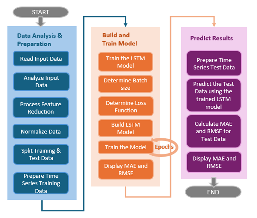
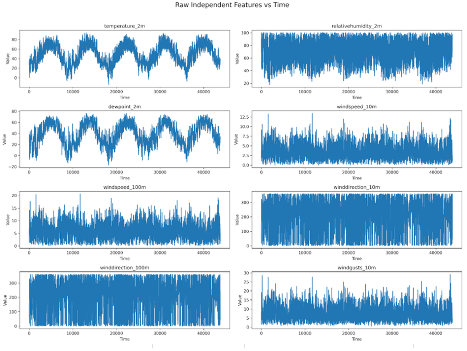
For the project Kaggle was used for the historical wind power generation figures, specifically the “Wind Power Generation Data – Forecasting” set put together by mubashirrahim²⁷. There are eight principal environmental variables in this dataset that serve as the independent ones; among them are temperature, humidity, and wind speed and direction. The table below details these features and their units, along with how they physically relate to power generation.

• Wind Speed (10 m and 100 m)
  • Units: meters per second (m/s).
  • Power output is a function of the wind speed cubed, making it the most important factor to monitor. A significant aspect is the 100 m measurement; being at the level of the turbine hub, it gives a true picture of the wind in an area where ground friction is no longer an impediment.
• Wind Gusts (10 m)
  • Units: meters per second (m/s).
  • These are brief, sharp surges in velocity that will put a spike on power production. On the other hand, should a gust surpass the cut-out speed, the turbine will engage its automatic shutdown to spare the machinery from damage, and output will fall off accordingly.
• Wind Direction (10 m and 100 m)
  • Units: degrees (0-360).
  • This dictates how the blades are positioned. One has to account for any local topography or wake effects from neighboring turbines that can impinge on efficiency when the direction changes.
• Temperature (2 m)
  • Units: degrees Fahrenheit.
  • Because cold air is denser and holds more kinetic energy than warm air moving at an equivalent pace, it is conducive to greater power generation.
• Dew Point (2 m)
  • Units: degrees Fahrenheit.
  • In addition to a minor effect on air density, an elevated dew point in colder weather is a warning sign for blade icing, which is hard on aerodynamic performance.
• Relative Humidity (2 m)
  • Units: percentage.
  • In much the same way as the dew point, humidity plays into the thermodynamics of the air. It is a component in determining both the lift on the blades and the overall air density.

Wind power output is the dependent variable here. There is data from four separate locations, but for the purposes of this study the model was trained and tested on Location 1 alone. The other three sites were left out of the train/test split entirely; they serve only as a fully held-out check of the model’s accuracy on unfamiliar ground to preclude any spatial leakage.

The dataset for each location comprises 43,800 hourly records with eight environmental features and a Power target, running from 00:00 on January 2, 2017 to 23:00 on December 31, 2021 (nearly five years). The data was divided 80/20 for training and testing, but did so in strict chronological order rather than at random. There is no shuffling involved: the first 80% of the time-ordered records are for training and the most recent 20% are reserved for testing. Once the 24-step look-back window is put in place (which eliminates the first 24 rows), the boundary for Location 1 falls at row 35,020. This yields a training set of 35,020 sequences from January 3, 2017 through 03:00 on January 1, 2021, and a test set of 8,756 hourly records covering the period from 04:00 that day to the end of 2021.

Data Preprocessing

Before training the model, every column was rescaled, including the Power target, to the [0, 1] interval with a Min-Max scaler. The scaler and the FeatureWiz feature-selection step were fit on the complete time series prior to the chronological split. While a more rigid approach would confine these to the training portion, the statistics of the held-out test period could have some bearing on the selected feature set and the scaler’s bounds.

A conventional sliding-window was used to build the 24-step look-back sequences. For any given time step t, the 24 preceding rows of scaled features (t−24 to t−1) are concatenated into an input vector from which the model must predict the current Power value. It is a one-step-ahead forecast (h = 1) since the reading from time step t is not part of the input. The processing pipeline does include an optional filter for outliers (z-score over 3) and a zero-power removal step, but both were left in their default off position for the results presented in this manuscript. As for missing sensor data, it was not imputed; the only rows discarded were the initial 24 of each location’s series, as they cannot form a complete lagged feature set.

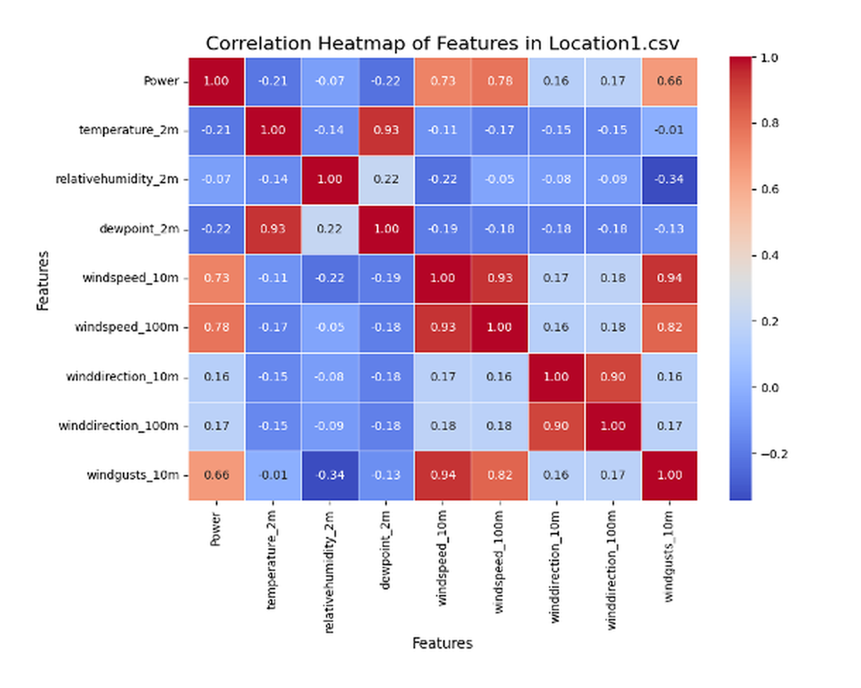
The initial dataset for Location 1 was put through a Pearson correlation analysis to better focus the model and improve its computational efficiency.

The heatmap shows that Power is most strongly and positively correlated with windspeed_100m (0.78), windspeed_10m (0.73) and windgusts_10m (0.66). In short, it is the wind velocity at different altitudes and any sudden gusts that are the main determinants of energy production. The linear relationship with such things as relativehumidity_2m (-0.07), dewpoint_2m (-0.22) and temperature_2m (-0.21) is far more tenuous, bordering on negligible.

With these statistics in mind, FeatureWiz carried out the dimensionality reduction required for the Reduced-Feature Model. This automated library applied its SULOV algorithm to settle on the more predictively important of any mutually correlated pairs (using a 0.95 limit), then ranked them recursively against the Power target. The process did away with winddirection_10m, winddirection_100m and relativehumidity_2m, leaving an input vector of five dimensions rather than eight.

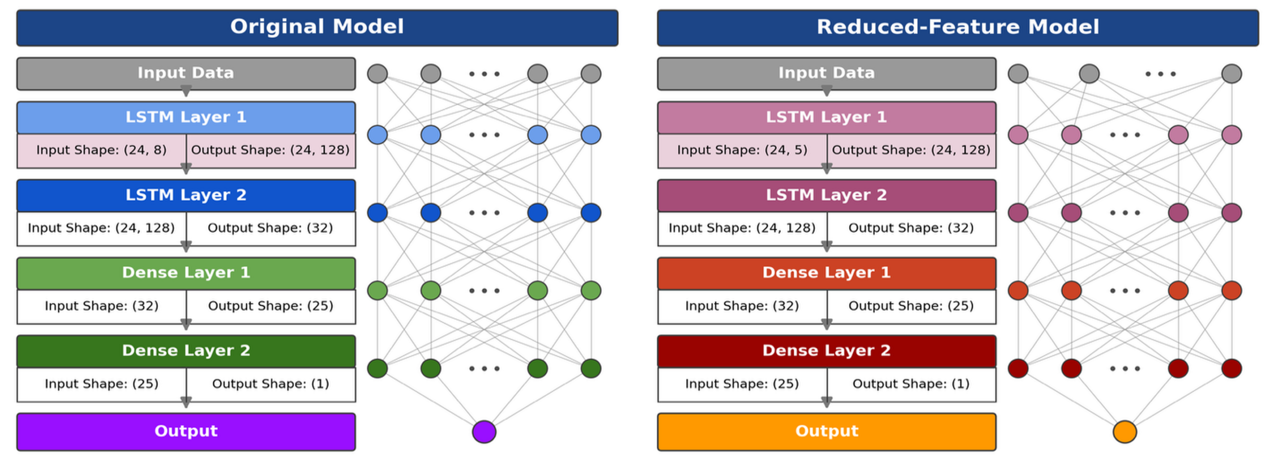
The wind power forecasting system is built on an architectural framework that is essentially a sequential hybrid model. Its purpose is to make use of specialized layers for the non-linear relationships and temporal dependencies found in the environmental data. The design is a four-layer affair: two Long Short-Term Memory (LSTM) units give way to two Dense layers, guiding the model from high-dimensional sequences down to a scalar output.

To begin, the first LSTM layer takes in an input of (24, 8) for the Original setup or (24, 5) for the Reduced-Feature one; the 24 being the hourly look-back window and the other figure denoting the feature count. Acting as a many-to-many processor, this initial stage projects the data into a 128-dimensional space so as to preserve its order and pull out any complex feature interactions. From there the representation is handed off to LSTM Layer 2. With an output shape of 32, this second layer is tasked with condensing the temporal information. A many-to-one approach is used to distill the 128-unit sequence into a more manageable vector of the key long-term patterns needed for a reliable forecast.

Once recurrent processing is complete, the model makes way for a feed-forward structure to carry out the final regression. The 32-unit vector put out by the LSTM block is taken in by Dense Layer 1 and mapped to an output of 25. In doing so, this layer refines the internal representation with non-linear transformations and puts the high-level LSTMs’ extractions into context. From there, Dense Layer 2 accepts the 25-unit input to yield a solitary output of 1, which is the predicted figure for wind power generation. It is a hierarchical reduction from a (24, 8) multi-featured sequence to a single prediction that enables the model to zero in on the variables behind energy output while filtering out environmental noise. A look-back window is employed to factor in the recent history of atmospheric conditions. Moreover, going from 128 units down to 1 is a matter of computational efficiency that does not come at the expense of the representations the model has learned.

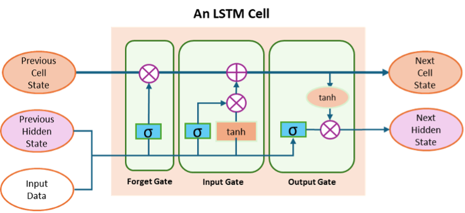
A standard recurrent neural network is prone to the vanishing gradient problem, an issue that the Long Short-Term Memory (LSTM) unit is built to counteract with its more complex internal design[1]. An LSTM cell takes in three separate inputs: the current input vector and both the hidden and cell states from the prior step. The latter of these serves as a form of “long-term memory,” an internal transport system that can convey information over long sequences with little in the way of linear interference. The former, the previous hidden state, is the “short-term memory” for localized temporal dependencies from the last step. As for the input data, it brings in exogenous variables like wind speed or temperature at the present time index.

The cell’s operation is controlled by three functional gates – the Forget, Input and Output – each a neural network layer with a sigmoid activation. This maps values on a 0 to 1 scale, acting as a filter where 1 means total retention and 0 is complete exclusion. In this way the model can learn to distinguish between environmental fluctuations of consequence to long-term power generation and the kind of stochastic noise best left behind to avoid overfitting.

The Forget Gate first comes into play to assess what historical data has any staying power. It concatenates the current input with the old hidden state and runs it through a sigmoid to see which parts of the previous cell state are no longer of use for the prediction. For wind power forecasting, this is essential to let go of weather patterns that have ceased to be a factor in the current atmosphere. A point-wise multiplication with the previous cell state then wipes the slate clean of such obsolete details.

Next, the Input Gate decides how much of the new information to fold into the long-term cell state. Here a dual-activation method is used: a hyperbolic tangent layer puts forward a candidate vector of new values, while a sigmoid layer vetoes or approves the significant features of the current input. The two are multiplied so that only the approved candidates are added to the modified cell state, yielding a current state that is a sound mix of relevant observations and enduring history.

To close out the cycle, the Output Gate is tasked with producing the hidden state for the time step. A tanh function is applied to the cell state to keep the values mathematically stable between -1 and 1, and a sigmoid layer picks out those elements of the updated state that matter for the prediction at hand. The final hidden state vector is the product of the two; it is put to work in the immediate power generation forecast and sent on as a recurrent input to the next layer, thus completing the processing of temporal information.

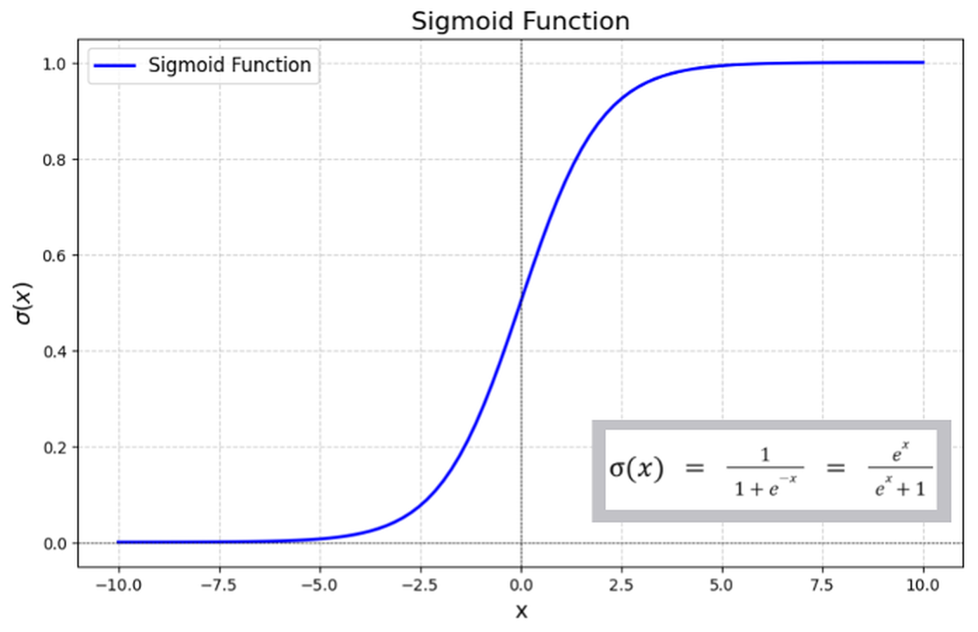
The model makes use of both functions in every LSTM cell. In the case of the forget, input and output gates, the sigmoid is the function of choice. With an output from 0 to 1, it serves to decide what gets through: a value near 1 means the time-series history is of high importance and must be kept, whereas something closer to 0 denotes information of little relevance.

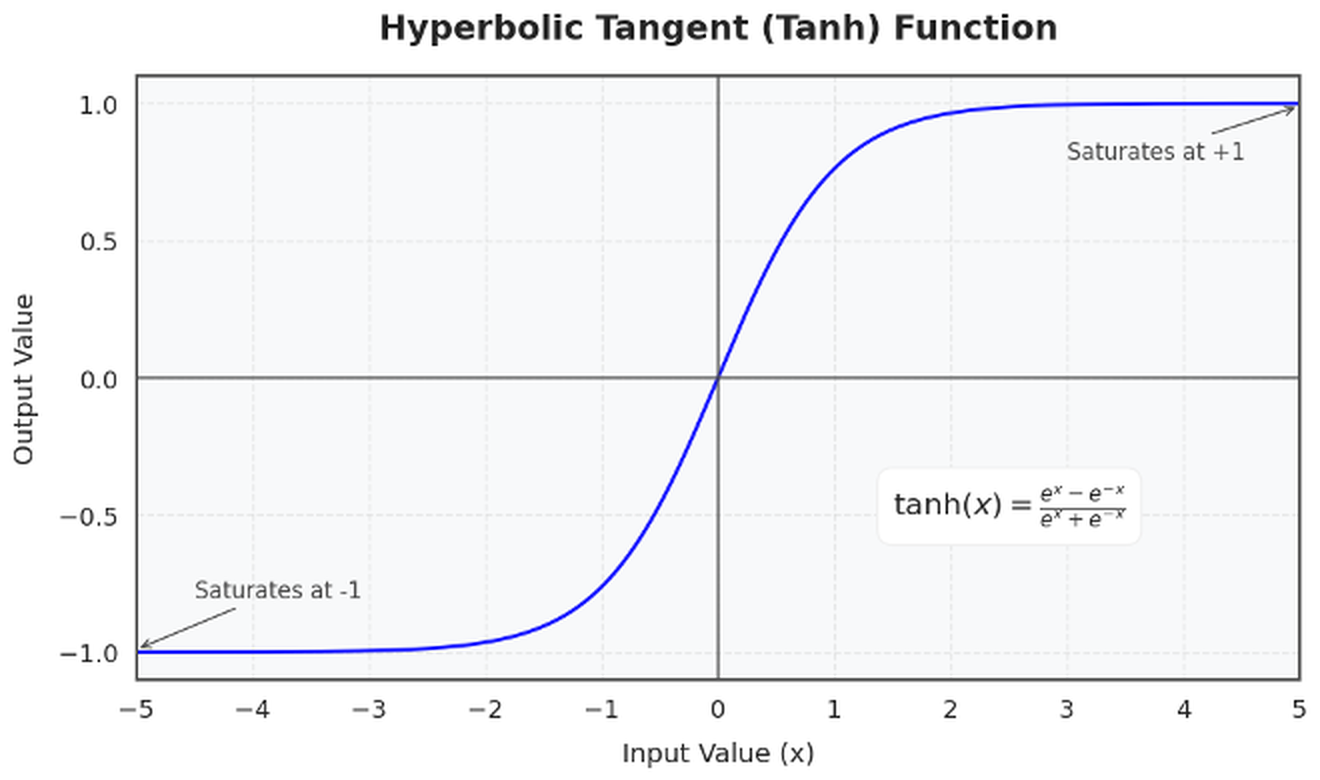
For the creation of a new candidate vector for the cell state and for scaling the final output, the tanh function is used. Because it yields values in the -1 to 1 interval, it is well suited to handle non-linearity and to center values around zero to regulate information flow. This proves especially advantageous in the input gate when one is scaling new information to be added to the cell state.

Results

This study demonstrates that the reliability and accuracy of deep learning models can be optimized for wind power forecasting with the right feature selection and the use of Long Short-Term Memory (LSTM).

The Original Model is set as the baseline and was trained in batches of 72 for 20 epochs to find the minimum loss and prevent overfitting. It achieved an RMSE of 0.01106 and an MAE of 0.00759, using an Adam optimizer, which was left at default 0.001 learning rate for this task. The errors appear to be very small since they are defined on a unitless 0-1 scale as the source data for the Power column is already bounded within [0, 1]. The Min-Max scaler in the preprocessing stage did not change the data much since, as mentioned previously, the power output was already bound 0 to 1.

The model takes into account the past 24 hours since grid operators require a notice at least 24 hours prior to properly plan for energy production and can accurately allocate different energy sources to the electrical grid.

The model utilizes the common funnel design LSTM forecasting models instead of testing multiple architectures and setups. The first LSTM layer has 128 units to learn all the detailed patterns from the 24-step input. Next, the second layer of 32 units compresses all the details into a short summary, allowing the model to learn complex patterns while also preventing. Finally, an intermediate Dense (25) layer adds one more nonlinear step before the regression head, after which Dense (1) outputs the final Power forecast.

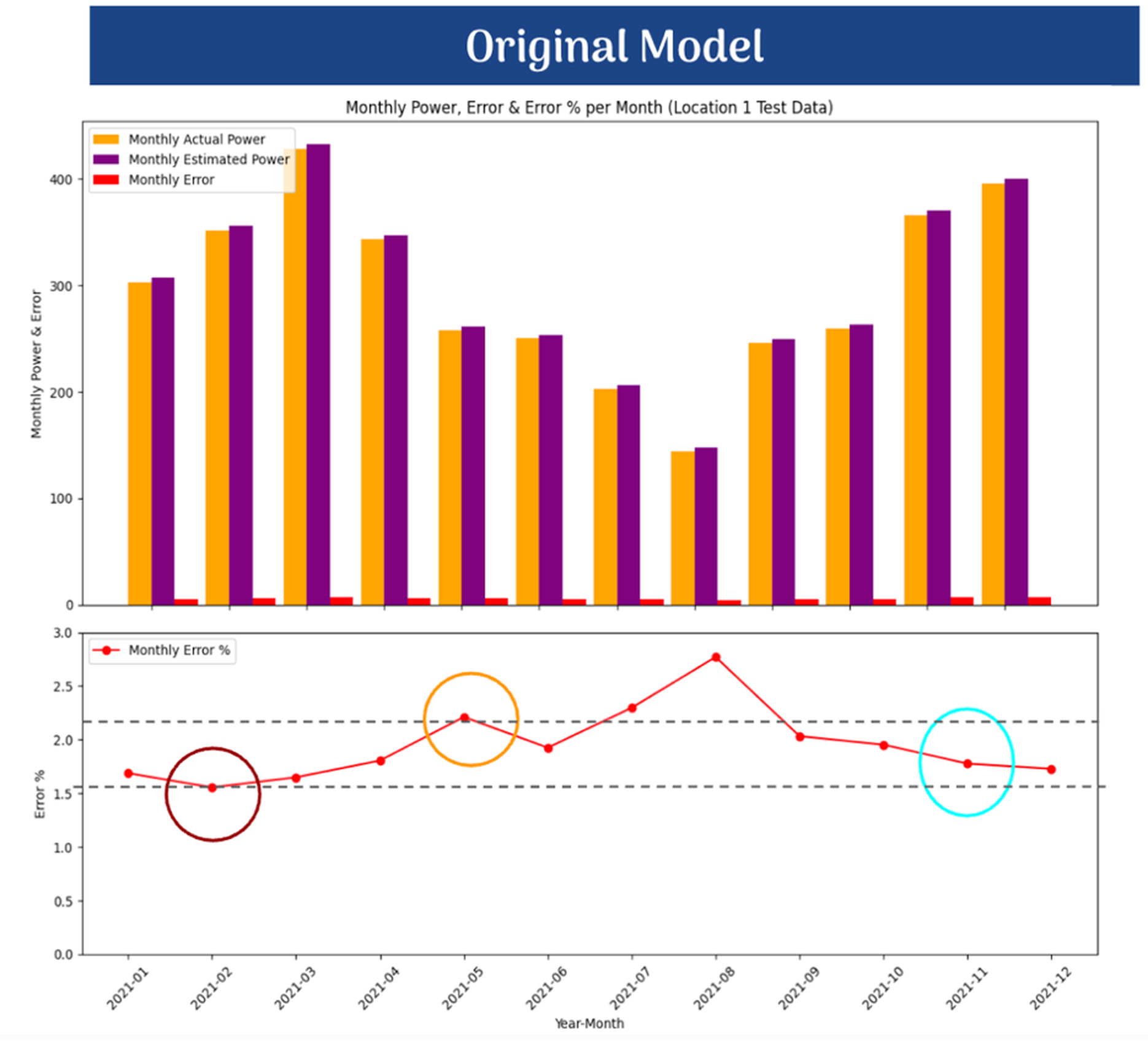
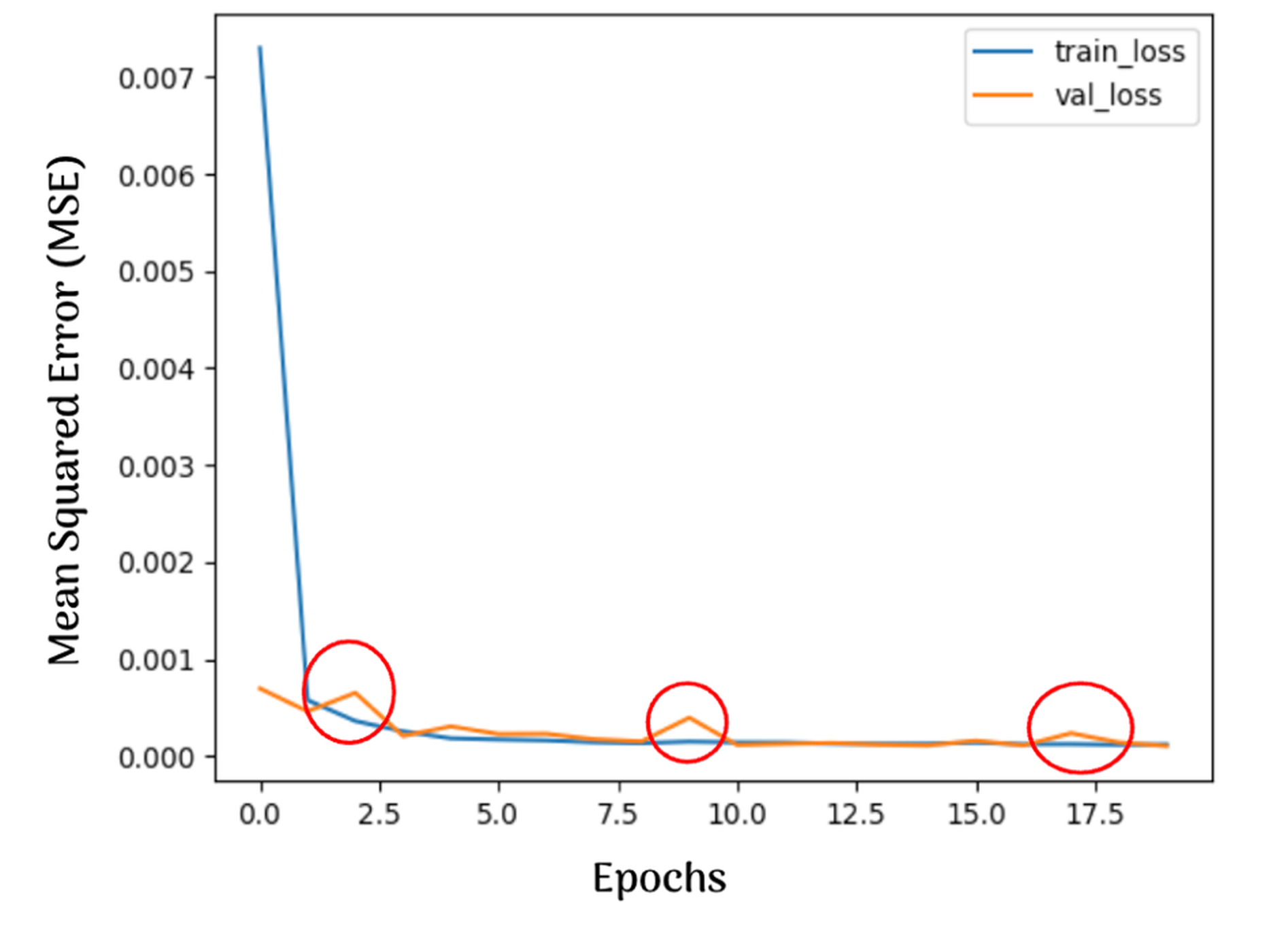
The model was effective as it was able to train in 4.10 minutes compared to the 5.75 minutes for the Kaggle reference model (Table 1). However, the Reduced-Feature Model showed even greater as the low-impact features were taken out and the environmental variables with a high correlation were put at a greater level of relevance. The resulting RMSE and MAE of 0.01006 and 0.00634, respectively, put the reduced-featured model ahead of the non-peer-reviewed LSTM model from Kaggle by 73.06% and 64.23% in terms of predictive accuracy.

The Kaggle community notebook was chosen as the comparative baseline since it incorporates the same dataset, feature set, and train/test split as the models in this study. As a result, any differences in accuracy, training time, and more can be attributed to this model’s architecture and feature selection and not be confounded with differences in the data. Other models mentioned in this paper, such as the C-LSTM of Wang et al. or the adaptive mixture-of-experts from Hossain et al., were originally put to the test on different wind farm data. In order to properly compare this study’s model with them, the entire architecture must be retrained with the data the prior models use as well as reprocess the data. The improvements gained over the Kaggle model represent a controlled comparison that shows the importance of reducing features.

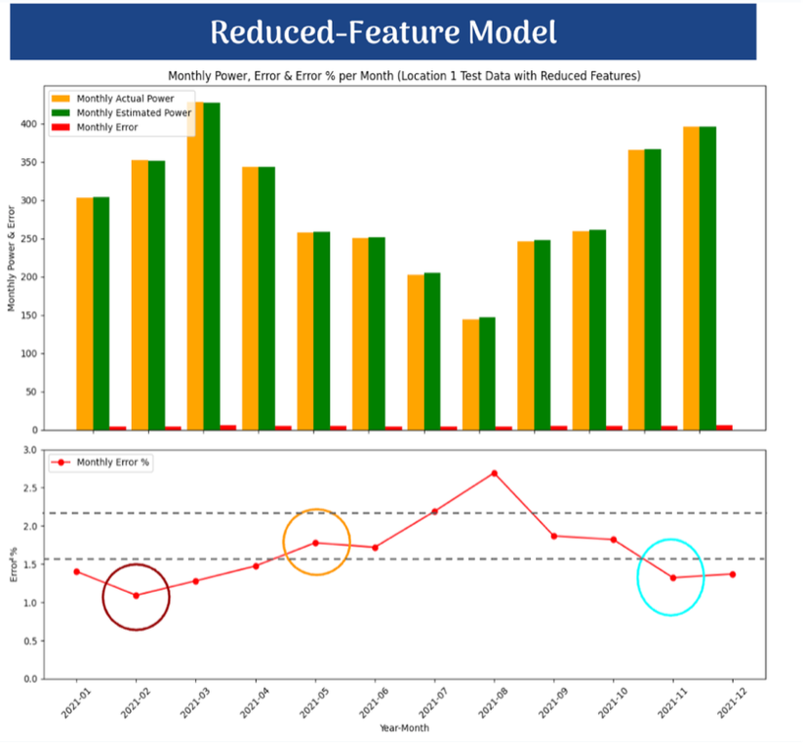
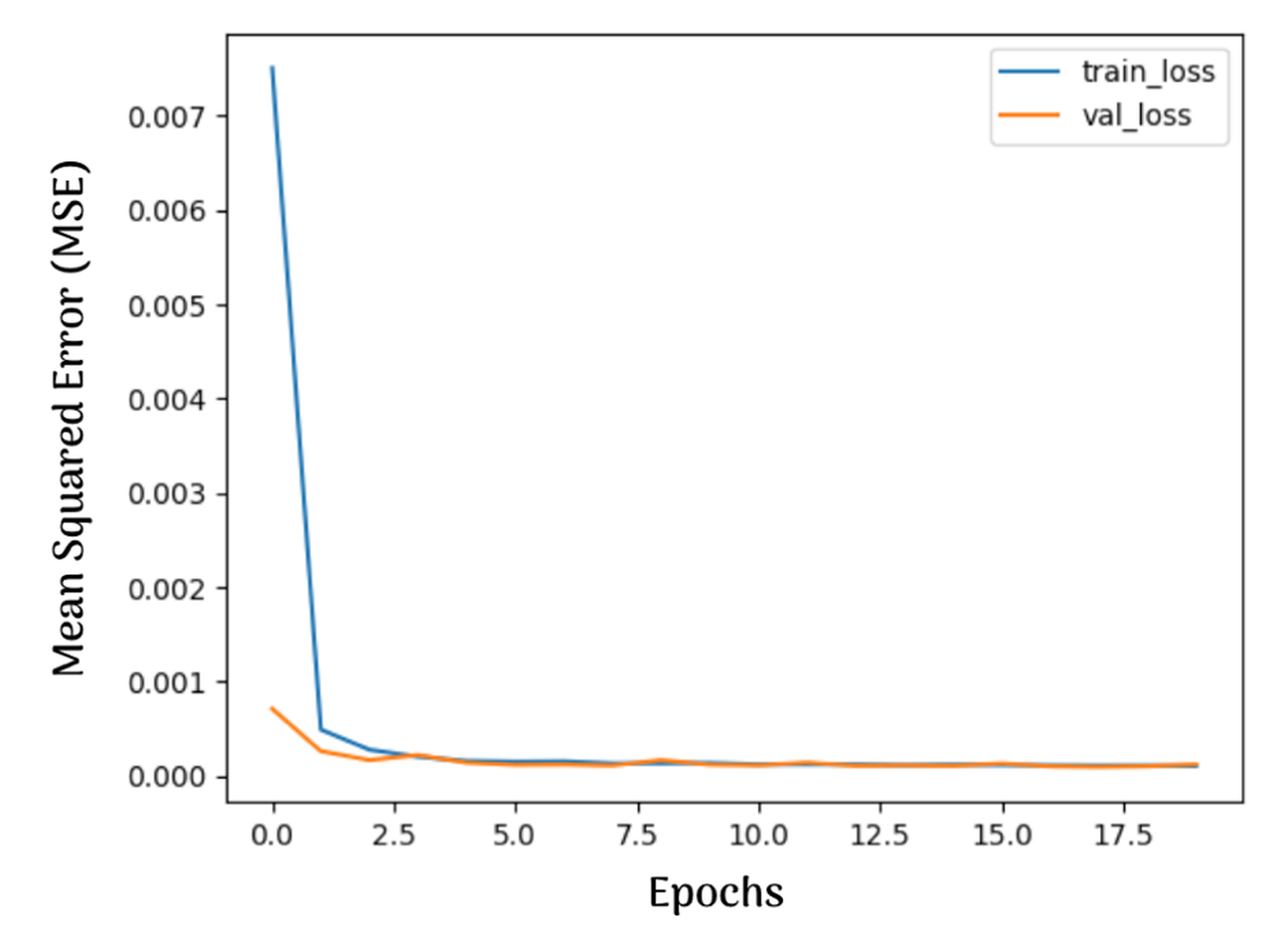
Part of the evaluation of the model also includes whether or not the computational performance is able to meet the need for utility applications to operate in real time. The Reduced-Feature Model, for instance, has a training time of 4.02 minutes, which is 30.12% faster than the 5.75 minutes achieved by the Kaggle reference model.

The work was done in PyCharm with TensorFlow 2.18.0 and the Keras API. All training and inference were run on the CPU of a Dell Precision 5530 (an Intel 8th Gen Core i7-8850H with 32GB DDR4 RAM and an Nvidia Quadro P1000 GPU). As a result, the error and running time figures in this study will be higher than what one would see from a GPU-accelerated system and cannot be fairly compared with studies that have access to such hardware. However, even without the acceleration, this processing speed combined with the model’s accuracy means it can be deployed in grid management to manage high-frequency data streams without the heavy costs and complexity of other deep learning tools.

	Ref LSTM Model	LSTM with 8 features	LSTM with 5 features
Training data (# features)	8	8	5
Training Time (seconds)	345.266	245.38	241.279
RMSE (Test data)	0.03734	0.01106	0.01006
MAE (Test data)	0.017726	0.00759	0.00634

The models trained on Location 1 were tested on completely unseen data of Locations 2, 3 and 4 to see how they would perform elsewhere without being retrained at all. The performance figures for each location, in terms of RMSE, MAE and total inference time, can be found in Tables 2 and 3.

The results show that both models still perform well at different locations, proving their generalizability. The Original Model’s RMSE (0.01009-0.01122) and MAE (0.00694-0.00755) at the unseen locations are roughly the same as its Location 1 error figures (RMSE 0.01106, MAE 0.00759), if not marginally superior by MAE. The Reduced-Feature Model, however, performed better and was able to generalize even more. Its unseen-location RMSE (0.00847-0.00943) and MAE (0.00540-0.00572) were lower than its own Location 1 test-set performance (RMSE 0.01006, MAE 0.00634). This suggests the five-feature reduction not only fits to the patterns of Location 1 but also transfers well to other sites. The Reduced-Featured Model also had a greater inference speed ranging from 9.34 to 9.95 seconds compared to the Original model, which ranged from 9.62 to10.72 seconds.

Unseen Data	Location 2	Location 3	Location 4
Unseen data (# features)	8	8	8
Inference time (seconds)	9.622	10.715	10.576
RMSE (unseen data)	0.01012	0.01122	0.01009
MAE (unseen data)	0.00720	0.00755	0.00694

Unseen Data	Location 2	Location 3	Location 4
Unseen data (# features)	5	5	5
Inference time (seconds)	9.335	9.627	9.949
RMSE (unseen data)	0.00847	0.00943	0.00860
MAE (unseen data)	0.00543	0.00572	0.00540

Discussion

For the modernization of electrical infrastructure, the findings here carry considerable practical weight. In giving utility firms a high-fidelity means of forecasting wind power generation, the work allows them to make exacting predictions on the ebb and flow of supply and demand. This in turn is beneficial for grid stability and does away with the requirement for carbon-heavy backup sources. In addition, with more accurate predictions of what the wind will produce, renewable resources are not needlessly put to waste and a greater share of that clean energy makes it to the end user. On a broader scale, the project puts forward a computational framework that is both efficient and scalable, one that supports the worldwide push to embrace renewables and cut emissions in the interest of a more sustainable and resilient energy landscape.

Limitations

There are a number of limitations that should be taken into account in the interpretation of these results. For one, the model’s generalizability to other parts of the world, be it different climates or turbine types, has not been established; it was put together and tested on nothing but a single Kaggle dataset (the Methodology section details how each of the four locations has 43,800 hourly records from Jan. 2, 2017 to the end of 2021).

As shown in Table 1 and Figures 8-11, the model was trained and tested only on Location 1, which is why the headline numbers for accuracy are reflective of Location 1 alone and not an aggregate of all four sites. As Tables 2 and 3 will show, the Original and Reduced-Feature models as-is were applied to the completely unencountered data from Locations 2, 3 and 4, with both showing good generalization. In the case of the Reduced-Feature Model, the RMSE and MAE for those unseen locations were consistently better than what was seen on the Location 1 test set.

The training was also confined to 20 epochs. Because the reported figures come from a solitary run, with no repeated trials to provide variance estimates or confidence intervals based on different random seeds, it is hard to say with certainty that the improvements are not down to some training noise. Finally, any claim of superiority is made against a non-peer-reviewed notebook from the Kaggle community rather than the kind of peer-reviewed forecasting work like C-LSTM or adaptive mixture-of-experts referenced in this paper, so the accuracy claims should not be over-generalized beyond that point of comparison.

Future Work

In the future, the model’s performance can be improved by tuning its settings more methodically instead of using the model’s defaults. For example, Bayesian optimization could have aided the model in finding the best possible learning rate and layers best suited to the model.

This model was able to reduce multicollinearity, but future version of it could incorporate even more data sources, such as live data or satellite images that can capture weather conditions that ground sensors potentially overlook. In addition, predicting it even further ahead (weeks or even seasons) would allow the model to take climate trends into account.

Finally, the power curve can be improved by adding data such as turbine maintenance logs or models to test how the physical turbine can affect the output.

Conclusion

This study compared a reduced-feature LSTM deep-learning model for short-term wind power forecasting with the full-feature model version and a Kaggle reference (which is not peer-reviewed but was run on the same data). Cutting the input features from 8 to 5 demonstrates that it yields a better training efficiency and predictive accuracy. These findings show that choosing the right features, as well as deciding which ones are relevant and important enough to retain, help improve an LSTM model’s performance while simultaneously minimizing costs. However, there are still many open questions as to whether the dataset is widely applicable enough to different locations, climates, and more.

Acknowledgements

I want to thank my research teacher, Dr. Zane Moore, for guiding me through this project, from the early stages of writing my research proposal to building and refining my model.

References

1. M. Ahmadi, L. Knorr, and H. Meschede, Improvement of wind power utilization through flexible operation of data center in wind parks, Renewable Energy. Vol 248, pg 123073, 2025, https://doi.org/10.1016/j.renene.2025.123073. [↩]
2. P. Veers, C. L. Bottasso, L. Manuel, J. Naughton, L. Pao, J. Paquette, A. Robertson, M. Robinson, S. Ananthan, T. Barlas, A. Bianchini, H. Bredmose, S. Gonzalez Horcas, J. Keller, H. A. Madsen, J. Manwell, P. Moriarty, S. Nolet, and J. Rinker, Grand challenges in the design, manufacture, and operation of future wind turbine systems, Wind Energy Science. Vol 8, no. 7, pg 1071-1131, 2023, https://doi.org/10.5194/wes-8-1071-2023. [↩]
3. S. K. Suraparaju, M. Samykano, J. R. Vennapusa, R. K. Rajamony, D. Balasubramanian, Z. Said, and A. K. Pandey, Challenges and prospectives of energy storage integration in renewable energy systems for NET zero transition, Journal of Energy Storage. Vol 125, pg 116923, 2025, https://doi.org/10.1016/j.est.2025.116923. [↩]
4. Y. Charabi and S. Abdul-Wahab, Wind turbine performance analysis for energy cost minimization, Renewables: Wind, Water, and Solar. Vol 7, no. 1, 2020, https://doi.org/10.1186/s40807-020-00062-7. [↩]
5. M. Krichen and A. Mihoub, Long short-term memory networks: a comprehensive survey, AI. Vol 6, no. 9, pg 215, 2025, https://doi.org/10.3390/ai6090215. [↩]
6. Z. Barath, P. Veres, and A. Banyai, Beyond traditional forecasting methods: evaluating LSTM performance on diverse time series, Mathematics. Vol 14, no. 5, pg 838, 2026, https://doi.org/10.3390/math14050838. [↩]
7. D. Wang, M. Xu, Z. Guangming, F. Luo, J. Gao, and Y. Chen, Enhancing wind power forecasting accuracy through LSTM with adaptive wind speed calibration (C-LSTM), Scientific Reports. Vol 15, no. 1, 2025, https://doi.org/10.1038/s41598-025-89398-y. [↩]
8. M. T. Hossain, J. Cai, J. Han, X. Han, and Z. Li, Mathematically-guided ultra-short-term wind power forecasting based on adaptive mixture of experts, Energy and AI. Vol 24, pg 100742, 2026, https://doi.org/10.1016/j.egyai.2026.100742. [↩]
9. S. Roga, S. Bardhan, Y. Kumar, and S. K. Dubey, Recent technology and challenges of wind energy generation: a review, Sustainable Energy Technologies and Assessments. Vol 52, pg 102239, 2022, https://doi.org/10.1016/j.seta.2022.102239. [↩]
10. A. Kumar, M. Z. Khan, and B. Pandey, Wind energy: a review paper, Gyancity Journal of Engineering and Technology. Vol 4, no. 2, pg 29-37, 2018, https://doi.org/10.21058/gjet.2018.42004. [↩]
11. Z. Liu, H. Guo, Y. Zhang, and Z. Zuo, A comprehensive review of wind power prediction based on machine learning: models, applications, and challenges, Energies. Vol 18, no. 2, pg 350, 2025, https://doi.org/10.3390/en18020350. [↩]
12. E. A. Manzano, R. E. Nogales, and A. Rios, A systematic review of wind energy forecasting models based on deep neural networks, Wind. Vol 5, no. 4, pg 29, 2025, https://doi.org/10.3390/wind5040029. [↩]
13. M. A. Khan, I. A. Khan, S. Shah, M. EL-Affendi, and W. Jadoon, Short-term wind power forecasting through stacked and bi directional LSTM techniques, PeerJ Computer Science. Vol 10, pg e1949, 2024, https://doi.org/10.7717/peerj-cs.1949. [↩]
14. W. Xu, Z. Shen, X. Fan, and Y. Liu, Short-term wind power prediction based on anomalous data cleaning and optimized LSTM network, Frontiers in Energy Research. Vol 11, pg 1268494, 2023, https://doi.org/10.3389/fenrg.2023.1268494. [↩]
15. M. Belletreche, N. Bailek, M. Abotaleb, K. Bouchouicha, B. Zerouali, M. Guermoui, A. Kuriqi, A. H. Alharbi, D. S. Khafaga, M. EL-Shimy, and E. M. El-kenawy, Hybrid attention-based deep neural networks for short-term wind power forecasting using meteorological data in desert regions, Scientific Reports. Vol 14, pg 21842, 2024, https://doi.org/10.1038/s41598-024-73076-6. [↩]
16. D. Ma, Y. Gao, and Q. Dai, LFformer: an improved transformer model for wind power prediction, PLOS ONE. Vol 19, no. 10, pg e0309676, 2024, https://doi.org/10.1371/journal.pone.0309676. [↩]
17. X. Su, J. Gao, K. Han, H. Kim, and H. Jung, Research on enhancing short-term wind power forecasting through feature fusion in a hybrid deep learning framework, Scientific Reports. Vol 16, pg 10043, 2026, https://doi.org/10.1038/s41598-026-40689-y. [↩]
18. Q. Zhong, L. Wang, and C. Huang, T-LSTM: a novel model for high-precision wind power prediction by integrating transformer and improved LSTM, Applied Sciences. Vol 16, no. 3, pg 1609, 2026, https://doi.org/10.3390/app16031609. [↩]
19. E. Ghanbari and A. Avar, Short-term wind power forecasting using the hybrid model of multivariate variational mode decomposition (MVMD) and long short-term memory (LSTM) neural networks, Electrical Engineering. Vol 107, no. 3, pg 2903-2933, 2025, https://doi.org/10.1007/s00202-024-02685-1. [↩]
20. W. Lu, Z. Lu, W. Liu, and Y. Cao, Series-core fusion based multivariate variational mode decomposition for short-term wind power prediction using multiple meteorological data, Forecasting. Vol 8, no. 1, pg 15, 2026, https://doi.org/10.3390/forecast8010015. [↩]
21. H. Mauladdawilah, M. Balfaqih, Z. Balfagih, M. Pegalajar, and E. Jadraque Gago, Deep feature selection of meteorological variables for LSTM-based PV power forecasting in high-dimensional time-series data, Algorithms. Vol 18, no. 8, pg 496, 2025, https://doi.org/10.3390/a18080496. [↩]
22. T. A. Rajaperumal and C. C. Columbus, Enhanced wind power forecasting using machine learning, deep learning models and ensemble integration, Scientific Reports. Vol 15, pg 20572, 2025, https://doi.org/10.1038/s41598-025-05250-3. [↩]
23. M. Abdelsattar, M. A. Ismeil, K. Menoufi, A. AbdelMoety, and A. Emad-Eldeen, Evaluating machine learning and deep learning models for predicting wind turbine power output from environmental factors, PLOS ONE. Vol 20, 2025, https://doi.org/10.1371/journal.pone.0317619. [↩]
24. A. Zabihi, V. B. Manur, Y. Dintakurthy, KRKV Prasad, P. Rene, and V. B. M. Krishna, Machine learning-based wind speed forecasting: a comparative study, Scientific Reports. Vol 15, pg 40866, 2025, https://doi.org/10.1038/s41598-025-24640-1. [↩]
25. X. Li, K. Li, S. Shen, and Y. Tian, Exploring time series models for wind speed forecasting: a comparative analysis, Energies. Vol 16, no. 23, pg 7785, 2023, https://doi.org/10.3390/en16237785. [↩]
26. F. W. Mugware, C. Sigauke, and T. Ravele, Evaluating wind speed forecasting models: a comparative study of CNN, DAN2, random forest and XGBOOST in diverse South African weather conditions, Forecasting. Vol 6, no. 3, pg 35, 2024, https://doi.org/10.3390/forecast6030035. [↩]
27. mubashirrahim, Wind power generation data – forecasting, Kaggle, https://www.kaggle.com/datasets/mubashirrahim/wind-power-generation-data-forecasting, 2023. [↩]