An Integrated Machine Learning System for Crop Stress Diagnosis Combining Convolutional Neural Networks, Thermal Stress Mapping, and Hydrological Forecasting

Brian Lee; Vishwas Tattala

NHSJS

An Integrated Machine Learning System for Crop Stress Diagnosis Combining Convolutional Neural Networks, Thermal Stress Mapping, and Hydrological Forecasting

By

Brian Lee, Vishwas Tattala

-

October 18, 2026

0

27

Read the full article as a PDF Download

Abstract

The engineering integration of the Crop Disease & Insect Classification, the thermal screening using CWSI (Crop Water Stress Index), GRACE Terrestrial Water Storage Anomalies (TWSA) and Soil Moisture models to produce a single integrated mobile application on approximately $400 worth of drone and sensor equipment has been completed. This research project focuses on demonstrating engineering integration and does not evaluate the effectiveness of this technology as it relates to its ability to be used in agricultural applications. The Crop-Disease Classifier and Insect Classifier were both trained on 578,340 images representing 311 different types of crops and 1,359,384 images representing 515 different species of insects. These Classifiers resulted in accuracies of 95.5% and 83.3%, respectively when tested internally on a single run. When the Crop-Disease classifier was tested externally in a single session using data from 500 real-world samples, it had an accuracy rate of 93.8% (95% Confidence Interval: 91.3%-95.7%). Similarly, the insect classifier was tested externally in a single session using data from 451 real-world samples and resulted in an accuracy rate of 90.2% (95% Confidence Interval: 87.1%-92.7%). The thermal screens developed as part of this project are currently not validated against any biological or physical “ground truth” and therefore represent an uncalibrated proxy until further studies can validate them. The GRACE TWSA component showed a strong positive correlation with actual values when temporally rerunning the data under safe conditions (r = .902), however due to the fact that it did not perform better than a simple persistence baseline, the results obtained during this phase of development are considered preliminary. As noted above, a leakage-safe offline rerun of the soil moisture sensor successfully met all predetermined performance criteria (Bias, Mean Absolute Error, Root-Mean-Squared-Error and upper bound of Root-Mean-Squared-Error) and demonstrated a minimum correlation coefficient (r ≥ .70). Therefore, while the soil moisture model provided the most compelling evidence of model validity, the controller that integrates these signals into the Water Agent’s risk context labels continues to use fixed seed demonstration inference instead of relying upon real-time observation inputs. Additionally, although the rule-based water agent was able to provide deterministic responses based upon input parameters, it was only evaluated for its deterministic response characteristics and parameter sensitivities, and not its agricultural relevance.

Keywords: precision agriculture, crop stress, plant disease classification, pest identification, thermal imaging, Crop Water Stress Index, terrestrial-water-storage-anomaly forecasting, soil-moisture prediction, drone-based sensing, TensorFlow Lite, decision support

Introduction

Acre Intelligence was created to evaluate if a variety of different sensor and predictive elements could be used together as part of a single mobile workflow. As such its contributions have been related to software integration versus providing valid diagnoses or interventions. In addition to having access to compiled images, evidence for Acre Intelligence has also included using an uncalibrated thermal proxy and evaluating hydrological development within four sub-regions in California and Michigan. Additionally the approximately $400 that is estimated as the cost for developing the Acre Intelligence prototype hardware represents only the cost for hardware, it does not include other costs associated with using the system including the cost of the phone(s), connectivity, hosting, maintenance, replacement parts and labor; nor do these estimates account for potential future commercial or subscription-based offerings. All evaluated elements in the Acre Intelligence application have been incorporated.

Literature Context

The peer-reviewed primary literature establishes the bounds of the evidence for each application area within this prototype. Leaf image studies, which are controlled, show that deep learning approaches can provide very accurate predictions when given large amounts of data. Studies at the field, aerial and lesion level (which were conducted in the field) examine issues associated with backgrounds, acquisition and domain shift effects¹’²’³’⁴’⁵. Studies using thermal cameras calibrate canopy temperatures to ground based or physiological measures (as opposed to treating an un-calibrated index as a diagnosis)⁶’⁷’⁸’⁹’¹⁰. Soils studies focus on native scale observations (e.g., cm vs. m), temporal structures (i.e., how soil moisture changes over time) and independent validation methods¹¹’¹²’¹³’¹⁴’¹⁵. Hydrologic studies are focused on separating components, establishing baselines and quantifying uncertainties related to hydrology¹⁶’¹⁷’¹⁸’¹⁹’²⁰. This body of work provided the basis for developing reporting and claim boundaries for this prototype; no study validates its accuracy, safety or potential value-added benefits in the field.

Methods

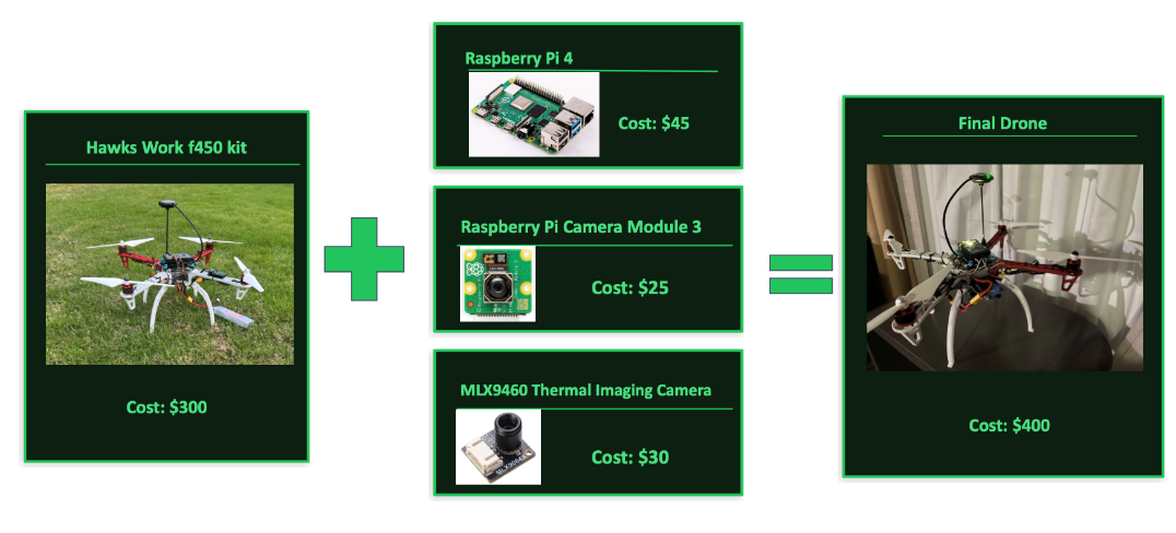
Figure 1 | Drone-mounted thermal sensing platform.

Cloud Backend hosting cost no money at all, as all services were hosted under the free plan on render.com

Thermal Stress Mapping

The thermal stress mapping system uses an MLX90640 infrared array sensor (24×32 pixels, 768 total readings) mounted on a Raspberry Pi 4, paired with the drone’s RGB camera. The sensor streams temperature readings over I2C at a refresh rate of 2 Hz, with each frame processed in real time. For each pixel (i,j) in the thermal frame, a leaf-air temperature delta is computed as:

\Delta T(i,j) = T_{\mathrm{leaf}}(i,j) – T_{\mathrm{air}}

A simplified, CWSI-inspired stress index is then calculated as:

\mathrm{CWSI}(i,j) = \frac{\Delta T(i,j)}{T_{\mathrm{opt,max}} – T_{\mathrm{air}}}

where ( $T_{opt,max}$ ) is a fixed crop-temperature constant used by the prototype. Unlike the original CWSI, which uses empirically determined non-water-stressed and non-transpiring baselines, the prototype applies the displayed equation directly. To prevent division by zero or sign inversion when ( $T_{\mathrm{air}} \geq T_{\mathrm{opt,max}}$ ), a software guard clause binds the denominator to a minimum threshold of 0.1 $^\circ$ C, ensuring mathematical stability in high-temperature regimes. Per-pixel values are aggregated to a field-level index using the equation:

\mathrm{CWSI}_{\mathrm{field}} = \frac{1}{768} \sum_i \sum_j \mathrm{CWSI}(i,j)

The thresholds utilized to sort pixels into their respective exploratory display bins were 0, 0.25 and 0.65. These threshold values were adapted from FAO guidance as initial reference points but were not derived from crop-specific physiological measurements in this study. These cutoffs have no validated biological meaning in this study and must not be used for field diagnosis until calibrated against independently measured plant water status indicators such as leaf water potential or stomatal conductance. Therefore, they should not be used for diagnostic purposes until each has been specifically calibrated for use in diagnosing drought conditions in each of the crop types studied and/or protocols utilized. Each pixel was sorted into one of four categories: actively transpiring (CWSI $<$ 0), healthy (0 $\le$ CWSI $<$ 0.25), mild stress (0.25 $\le$ CWSI $<$ 0.65) and severe stress (CWSI $\ge$ 0.65). Spatial associations of stress throughout the thermal field can also be assessed through the utilization of Moran’s I²¹, which computes the autocorrelation among the per-pixel CWSI values at every time point as a fast statistical filter to distinguish nonrandom spatial patterns from background noise:

I = \frac{N}{W} \frac{\sum_i \sum_j w_{ij}(\mathrm{CWSI}_i – \overline{\mathrm{CWSI}})(\mathrm{CWSI}_j – \overline{\mathrm{CWSI}})} {\sum_i(\mathrm{CWSI}_i – \overline{\mathrm{CWSI}})^2}

Moran’s I takes into account spatial adjacency weights ( $w_{ij}$ ) (i.e., how close together pixel i and pixel j are) so it can quantify if an area with higher CWSI values are clustered or spread out, while a p-value is used to determine if this is statistically significant from random chance. The prototype uses a very strict definition for flagging frames for stress-zone rendering – statistical significance (p $<$ 0.05). In contrast, the absolute value of Moran’s I has no biological basis for defining the extent of physiological stress in plants. Therefore, the choice of p = 0.05 is not related to any labeled physiological stress zones within the images taken, nor is the biological significance of the resulting clusters understood at present. Within flagged regions, boundaries between stressed and healthy areas are identified using a discrete Laplacian operator:

(T*K)(i,j) = \sum_m \sum_n T(i+m, j+n)\cdot K(m,n)

computed as the second-order spatial derivative of the temperature field:

\nabla^2T(i,j) = T(i+1,j) + T(i-1,j) + T(i,j+1) + T(i,j-1) – 4T(i,j)

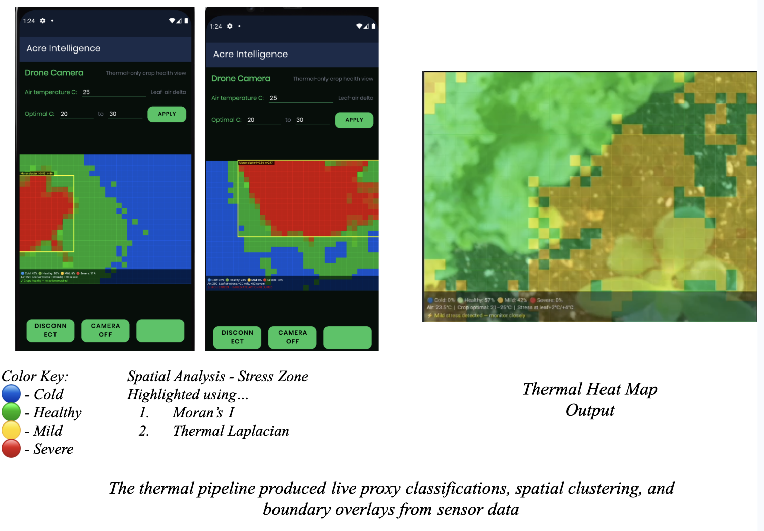
Pixels where ( $|\nabla^2T|$ ) exceeds a fixed threshold are marked as boundary pixels and rendered as an overlay on the thermal heat map to indicate the spatial extent of detected clustering regions. A fixed display value (threshold) of 2.0 $^\circ$ C was chosen as the Laplacian Threshold a priori for visualization purposes to clearly separate distinct spatial areas of interest, as opposed to a physiologically meaningful boundary. The entire system from data collection, through CWSI inspired classification to Moran’s I spatial autocorrelation analysis using an associated p-value test, then to producing a real-time heat map overlay within the app via Laplacian Boundary Display is performed on device without utilizing outside cloud-based services or network connectivity.

Plant Disease Classification & Insect Classification

Research Design

Disease and insect classification used comparative model development. Disease candidates included logistic regression, SVM, MobileNetV2, ResNet50, and a custom CNN; insect candidates included KNN, random forest, VGG16, EfficientNet, and a transfer-learning CNN. Custom CNN variants were selected for their accuracy-efficiency tradeoff.

Sample & Data Collection

No humans or animals were involved in this study. The plant disease dataset comprised 578,340 images and 311 disease categories, obtained from 2 Kaggle collections — “New Plant Diseases Dataset” at https://www.kaggle.com/datasets/vipoooool/new-plant-diseases-dataset and “Plant Disease Dataset,” also available on Kaggle (https://www.kaggle.com/datasets/emmarex/plantdisease), along with images scraped using an additional python-based scripting tool. Each class had between 1,659 to 2,109 images. The insect classification dataset contained 1,359,384 images categorized into 515 different insect species and came from 2 Kaggle collections — “Insects Dataset” at https://www.kaggle.com/datasets/ismail703/insects and “Dangerous Insects Dataset” at https://www.kaggle.com/datasets/tarundalal/dangerous-insects-dataset — and was further enhanced through images scraped using the PkSu image scraping technique. Each class contained between 1,659 to 2,679 images. Duplicate images (exact and near duplicate) were deleted before each dataset was separated into training and testing partitions. Since all images of a particular type of plant or insect existed in only one partition, the partitions were separated based on specimens, eliminating potential cross-partition information flow. The approximate ratios of train to test for both datasets were approximately 4.06 to 1 (disease) and 4.01 to 1 (insect). It is recommended that the individual rights and restrictions associated with all components of these datasets be evaluated separately prior to utilizing the datasets in research or distributing any resultant products commercially.

Variables and Measurements

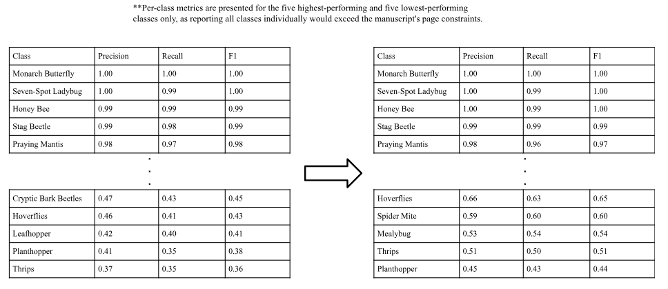
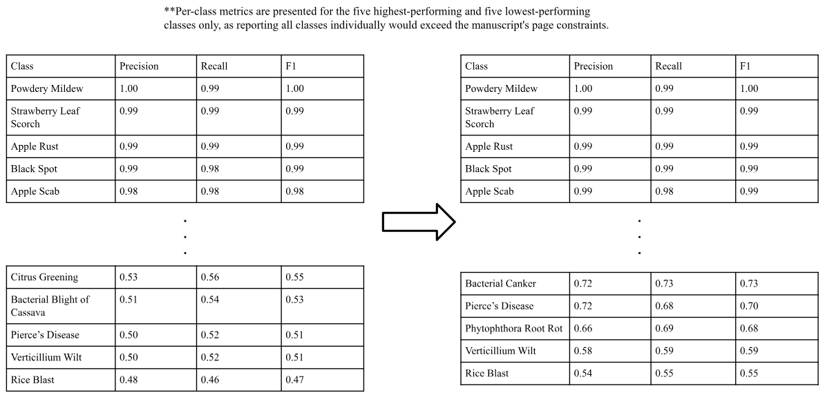
Model architecture was the independent variable. The primary outcomes (for both models) were cross-entropy loss and held-out accuracy. Top-5 insect classification accuracy was also recorded. For all classes, precision, recall, and F1 score were calculated and then summarized using macro and weighted averages of these scores. The top-5 and bottom-5 performing classes by F1 score are reported in the Results section.

Procedures

For both models, the final classification layer applies a softmax function to convert raw output scores into class probabilities. For an input x, the probability that x belongs to class k is given by:

P(y = k \mid x) = \frac{e^{z_k}}{\sum_{j=1}^{K} e^{z_j}}

where ( $z_k$ ) is the raw output score (logit) for class (k), (K) is the total number of classes (311 for the disease model, 515 for the insect model), and (j) indexes over all classes. The predicted class is the one with the highest resulting probability.

Class imbalance across the 515 insect species was operationalized through a class-weighted cross-entropy loss:

L_w(\theta) = -\sum_{k=1}^{515} w_k y_k \log(\hat{y}_k)

where ( $\theta$ ) represents the model’s parameters, ( $y_k$ ) is the true label for class (k), and ( $\hat{y}_k$ ) is the predicted probability for the class (k) from the softmax output above. The weight is computed as:

w_k = \frac{N}{K \cdot N_k}

The impact of class weights on detection rates for rare species were evaluated by comparing the per-class precision, recall, and F1 for the 5 lowest ranked species between the two training configurations. The results of this comparison can be found in the Results section. Horizontal flip, rotation up to ±30°, and brightness shift ±20% are the three transformations that make up the disease augmentation. Class weights plus minority oversampling, majorities undersampling, batch normalization and drop-out (probability=0.5) are the four techniques employed during insect training. For inference on mobile devices with minimal latency (measured at .05 – 1.0 second), both models have been converted into INT8 TensorFlow Lite²². These conversions resulted in a model size reduction of approximately four times their original sizes. To assess training stability, both models were retrained five times from scratch using different random seeds; the standard deviation of test accuracy was 2.3% for the disease model and 2.7% for the insect model, indicating reasonable stability across initializations.

Participants, Samples, and Study Units

Beginning with study units, samples and participants, there were no human participants in this research. The GRACE TWSA model was developed using bounding box files for California and Michigan. Those two states were further divided by the android user interface into California North, California South, Michigan Upper and Michigan Lower request labels. However, those labels do not represent that the GRACE TWSA model has been trained regionally and independently.

Data Collection and Instruments

The data collection instruments and methods included the use of GRACE TWSA JPL GRACE/GRACE-FO Mascon RL06.3Mv04 CRI liquid-water-equivalent thickness (lwe_thickness) on a 0.5 degree grid which represents approximately 3 degrees of an area of the Earth. There are 253 time-steps in the file provided containing lwe_thickness from 2002 thru 2026. The array size for each of the two states was different: California created 20 x 20 arrays while Michigan created 14 x 16 arrays. The outer aligned arrays created a combined 32×36 domain. Additionally, the GRACE TWSA development utilized a separate dataset, SoMo.ml v1 Layer 1 daily 0-10 cm volumetric soil moisture on its native 0.25 degree grid.

The primary dependent variables in this research project were the next GRACE terrestrial-water-storage-anomaly grid and the next soil-moisture grid. Six prior 32×36 grids composed the input of the GRACE TWSA and five prior 32×32 grids formed the input of the soil-moisture. The outputs were either continuous grids or interface categories. No subtraction of other storage components such as soil moisture, snow or surface water was made by retained code; hence the GRACE output is reported as TWSA and not as direct measurements of groundwater storage.

In addition to the retained codes previously mentioned, the live context of U.S. Geological Survey (USGS) well-depths was converted to a very minor display bias: i.e., average depth greater than 120 feet resulted in -0.13, greater than 70 feet results in -0.07, less than 25 feet resulted in +0.08 and all other valid depths results in +0.03. Furthermore, soil live context added +0.025 to the display bias whenever SMAP granules were present and -0.025 to the display bias when the GRACE TWSA display bias was at or below -0.08; the resulting value was then clipped to [-0.12, 0.12] to provide a form of contextualization to the maps being displayed as well as to interpretive actions taken by the agent.

GRACE TWSA Model Procedure

The supplied GRACE file was opened with xarray, longitude was converted to −180° to 180°, and lwe_thickness was clipped to [−100,100] cm liquid-water-equivalent thickness. California (32–42°N, 124–114°W) and Michigan (41–48°N, 90–82°W) were selected. Their natural 20×20 and 14×16 arrays were outer-aligned by coordinate to a 32×36 domain, creating padding that the development notebook filled with zero. No 32 × 32 interpolation was used for this GRACE TWSA artifact.

x_{\mathrm{clean}} = \operatorname{clip}(\operatorname{nan\_to\_num}(lwe_{\mathrm{thickness}}, 0), -100, 100)

X_{\mathrm{aligned}}(t) \in {R}^{32 \times 36}

Overlapping six-step input windows converted each state sequence into supervised samples:

X_i = [x_t, x_{t+1}, x_{t+2}, x_{t+3}, x_{t+4}, x_{t+5}], \qquad y_i = x_{t+6}

X \in {R}^{494 \times 6 \times 32 \times 36 \times 1}, \qquad y \in {R}^{494 \times 32 \times 36}

The development notebook calculated one global mean and standard deviation after combining both state series and before the train/test split. Consequently, test information entered preprocessing and the resulting development metrics are leakage-prone.

\mu_{\mathrm{dev}} = \operatorname{mean}(X_{\mathrm{all}}), \qquad \sigma_{\mathrm{dev}} = \max[\operatorname{std}(X_{\mathrm{all}}), 10^{-8}]

X^* = \frac{X – \mu_{\mathrm{dev}}}{\sigma_{\mathrm{dev}}}, \qquad y^* = \frac{y – \mu_{\mathrm{dev}}}{\sigma_{\mathrm{dev}}}

The 494 overlapping windows were randomly split 80:20 after window generation with random_state=42, producing 395 training and 99 test windows. This development split allowed adjacent overlapping sequences to cross partitions and is not confirmatory evidence.

CNN-LSTM pipeline: TimeDistributed Conv2D(16,3×3,ReLU,same) → TimeDistributed MaxPool2D(2×2) → TimeDistributed Flatten(4608) → LSTM(64)²³ → Dense(1152) → Reshape(32×36).

The saved Keras model contains 1,271,328 trainable parameters and was trained for 20 epochs with batch size 8 using Adam²⁴ (learning rate 0.001), mean-squared-error loss, and MAE monitoring. Its input shape is (None,6,32,36,1) and output shape is (None,32,36).

\mathrm{MSE} = \frac{1}{n} \sum_{i=1}^{n} (y_i – \hat{y}_i)^2

\mathrm{MAE} = \frac{1}{n} \sum_{i=1}^{n} |y_i – \hat{y}_i|

\theta_{t+1} = \theta_t – \alpha \frac{\hat{m}_t}{\sqrt{\hat{v}_t} + \epsilon}

The user had already generated an inference using the REST Backend that Grace TWSA deployed. Then the Android app would send both the “Region” and “Time”, and receive the “Status”, “Trend”, and “Heatmap” fields from Grace TWSA. NASA CMR²⁵’²⁶ and USGS²⁷’²⁸ supplied display context only; they did not convert GRACE total-water-storage anomaly into independently validated groundwater storage. A review of the Ground Water Predictor Project (retained Ground Water Predictor Android project) confirmed that this client (java/androidx targeting Android API 34 min api 24) utilized Retrofit/Gson serialization. The GRACE TWSA Client will transmit the Region, Time Range, Start Date, and End Date to the Deployed GRACE TWSA Service, and render the returned status, trend heat map fields. Although a pre-built debug APK is retained, there are no device logs or reproducible performance testing reports; therefore, no claims can be made regarding the new Android latency or success rates.

Soil-Moisture Model Procedure

Development utilized 20 annual SoMo.ml v1 Layer 1 NetCDF data files for the years 2000 – 2019. Data included layer 1, which contains daily volumetric soil moisture at 0-10cm depth in m3/m3 on a native .25 degree grid. For both California and Michigan, approximately the first 150 time-steps were extracted from each netcdf file. Non-finite values are assigned an arbitrary value of zero. Fields were then casted into a float32 format. Both California (.25 x .25 degree grid, approx. 40 x 44 pixels) and Michigan (.25 x .25 degree grid, approx. 32 x 32 pixels) grids were downsampled using a reflect mode, anti-aliasing method to create two new grids that were also 32 x 32. Using this approach five consecutive daily frames were trained to predict the next day’s frame creating training input sizes X = (5800, 5, 32, 32, 1) and output size y = (5800, 32, 32, 1). The network comprised Conv3D²⁹ layers with 16 filters (3x3x3, ReLU, same; 448 parameters), 32 filters (3x3x3, ReLU, same; 13,856 parameters), and one linear filter (1x1x1, same; 33 parameters), followed by selection of the final temporal slice. All 14,337 parameters were trainable. The training process utilizes the Adam optimizer and mean squared error loss function. It monitors mean absolute error loss during training. Training was conducted over ten epochs and the batch size was eight. Because the original development utilized standardized combined inputs and created overlapping windows prior to splitting it into a training/test sample ratio of 80:20, it will be shown here solely as a training diagnostic tool.

\hat{S}_{t+1} = f_{\theta}(S_{t-4}, \ldots, S_t)

The floating point 32-bit frozen model was converted to tensorflow lite format with the TensorSpec as follows (input) None x 5 x 32 x 32 x 1 and (output) None x 32 x 32 x 1 and the byte size of the artifacts were 60748 bytes. An android controller provides a static, pre-processed seed number, and min/max normalizes the forecasted grid to the range [0,1] in order to generate an image/heatmap from the forecasted data. The android controller will not provide any live raster observations (or download them).

Application Integration and Decision Agent

The system used by GRACE TWSA was utilizing cloud-based inference, whereas soil moisture was using on-device, fixed-seed inference. For the purposes of this prototype’s scoring, GRACE TWSA interface state and soil-moisture state were mapped into an aggregate risk-context label. Confidence levels were dependent upon availability of both signals: two signals = high; one signal = medium; none = no model data. While the Water Agent itself has remained non-prescriptive in terms of irrigation or treatments because it is a research prototype, the entire process of defining all input selections and rule development completed by the project team was developed through their own self-directed online research and/or engineering judgment. Neither an agronomist, irrigation specialist, hydrologist, extension professional nor any other independent domain expert participated in the design, calibration or approval of the architecture. The USDA-NRCS irrigation guidelines³⁰, FAO CROPWAT documentation³¹ and USGS drought/groundwater information³² were reviewed by the project team for directional relevance related to soil moisture, water balance context and TWSA trend analysis, although the project team defined all of the weights, cutoff values, and thresholds through their own developed heuristics rather than those derived from these documents. NIST AI RMF, EFSA expert-knowledge guidance, STARD and Fleiss’ agreement framework³³’³⁴’³⁵’³⁶ guided the reporting categories for this audit as well as for the proposed future validation designs; however, none of these resources guided whether the model is correct or incorrect. Outputs from the model are for demonstration purposes only as proof-of-concept software and as examples for research discussions; therefore outputs should not be used as operational advice (i.e. irrigation advice, pesticide application advice, crop-treatment advice). Weights and priority cutoff values were varied by ±1. Additionally, monotonic relationships were evaluated. This audit evaluates deterministic behavior and parameter sensitivity only; therefore, it establishes neither agronomic correctness, treatment safety, expert agreement, sensitivity/specificity, nor field benefit.

z_{\mathrm{norm}} = \frac{z – z_{\min}}{z_{\max} – z_{\min} + \epsilon}

\mathrm{Risk} = w_G G_{\mathrm{risk}} + w_S S_{\mathrm{risk}} + w_R R_{\mathrm{risk}}

w_G + w_S + w_R = 1

Data Analysis, Validation, and Reproducibility

Confirmatory soil-moisture analysis reported bias, MAE, RMSE, ubRMSE, Pearson correlation, baseline improvement, temporal block-bootstrap uncertainty, and TFLite parity. The retained GRACE TWSA analysis is reported separately.

Ethical Considerations: No human or animal subjects or identifying research data were used. Optional device location is an application feature.

System	Primary data	Model input	Output	Deployment
GRACE TWSA	GRACE/GRACE-FO + USGS/CMR context	6×32×36×1 grids	Next grid, status, trend, heatmap	Cloud CNN-LSTM REST backend
Soil moisture	SoMo.ml v1 Layer 1 + CMR/USGS context	5×32 × 32×1 grids	Next grid; Dry/Moderate/Wet	On-device TFLite
Water Agent	Two model states	Categorical/continuous outputs	Risk-context labels	Rule-based Android layer

Table 1 | Final water model and deployment configuration.

The soil-moisture splits, random seed, and evaluation checks are documented as development evidence; no treatment advice or preregistration claim is made.

Results

*Figure 2 | (Left) Plant-disease actual-versus-predicted plot.*

*Figure 3 | (Right) Insect-classification actual-versus-predicted plot.*

*Figure 4 | Insect-classifier per-class precision, recall, and F1 comparison.*

*Figure 5 | Plant-disease classifier per-class precision, recall, and F1 comparison.*

*Figure 7 | Insect-classifier summary metrics.*

*Figure 8 | Plant-disease classification diagnostic outputs.*

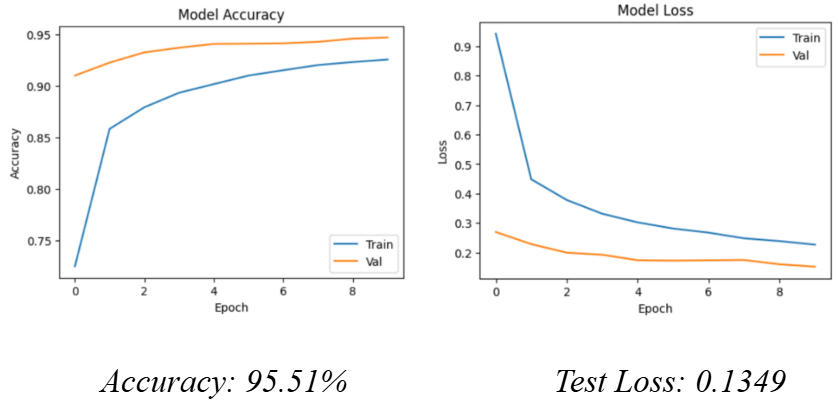
The disease model produced 95.51% single-run internal accuracy with test loss 0.1349.

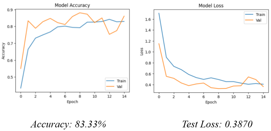
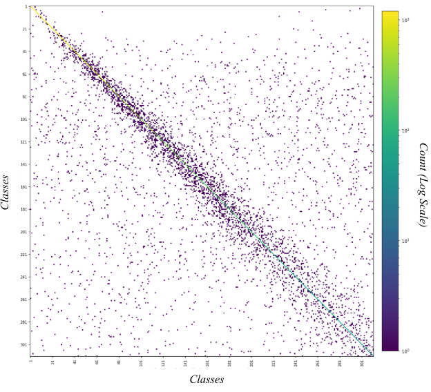
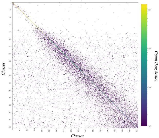
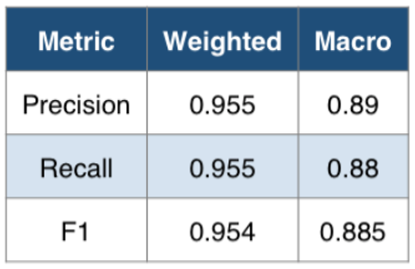
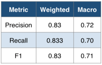
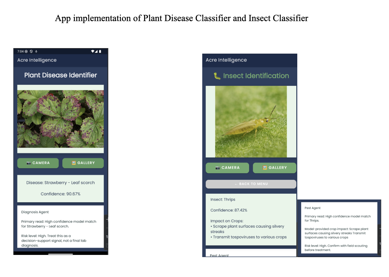
*Figure 9 | Insect-classification diagnostic outputs.*

The insect model produced 83.33% single-run internal accuracy with test loss 0.3870. Performance metrics for each model are summarized in the images included below. Figure 2 displays the relationship between actual and predicted values for disease (Figure 2), and insects (Figure 3). Tighter clustering along the diagonal indicates higher overall accuracy for disease models. Precision, recall, and F1 metrics are provided for the top five classes and bottom five classes of each model’s most accurate classifications in Figures 4 (insects) and 5 (disease). As would be expected, precision, recall, and F1 metric values near one are reported for the best performing classes while dramatically lower values were reported for the worst performing classes. This pattern of error concentration in specific hard-to-classify/rare classes is also visible when reporting weighted and macro averages of precision, recall, and F1 metric values in Figures 6 and 7. For example, the disease model reached a weighted average of 0.955/0.955/0.954 in terms of precision/recall/F1 metric values and a macro average of 0.89/0.88/0.885. Similarly, the insect model reached a weighted average of 0.83/0.833/0.83 and a macro average of 0.72/0.70/0.71 in terms of precision/recall/F1 metric values. The larger weighted-macro gap for the insect model reflects the wider spread seen in its per-class breakdown (Figure 4) as well as its larger number of classes (515 vs. 311). The same disease-over-insect performance gap seen above can also be observed when looking at training diagnostic data in Figures 8 and 9 where it is shown that the disease classifier achieved a single run test accuracy of 95.51% using a test loss of 0.1349 and the insect classifier achieved a single run test accuracy of 83.33% using a test loss of 0.3870. These internal estimates were supported by external field evaluations: the disease classifier correctly identified 469 of 500 real field images (i.e., a true positive rate of 93.8%) using a confidence interval of 95%. Additionally, the insect classifier correctly classified 407 out of 451 images used to evaluate the models spanning across thirty-one species sourced from Nature’s Good Guys (a true positive rate of 90.2%) with a confidence interval of 95%. It should not be interpreted broadly as validation across all classes and conditions because both evaluations represent only a single collection session.

*Figure 10 | Thermal stress mapping output.*

*Figure 11 | Integrated plant-disease and insect-classification output.*

Water Resources

Water components passed development and integration checks. Soil moisture additionally used chronological and complete-region holdouts with explicit baselines.

GRACE TWSA Forecasting Results

The provided GRACE TWSA artifact is an LSTM-CNN of 20 epochs and not a convolutional neural network with three dimensions (Conv3D) of 10 epochs. The originally leakage-prone 99 window development test was conducted with normalized MSE 0.071364, and normalized MAE 0.117362. Both of these metrics are for the purpose of software development testing; therefore, they are neither in physical units nor scaled as native or leakage-safe TWSA accuracy.

Figure 12 | GRACE TWSA CNN-LSTM development training and validation curves across 20 epochs. Because global preprocessing and overlapping-window random splitting preceded evaluation, these curves document optimization behavior only.

*Figure 13a | Predicted vs. actual GRACE TWSA.*

*Figure 13c | Absolute-error distribution.*

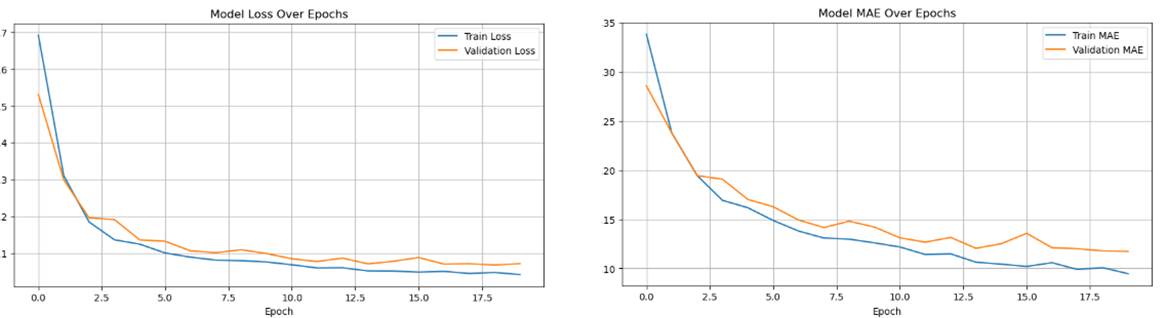
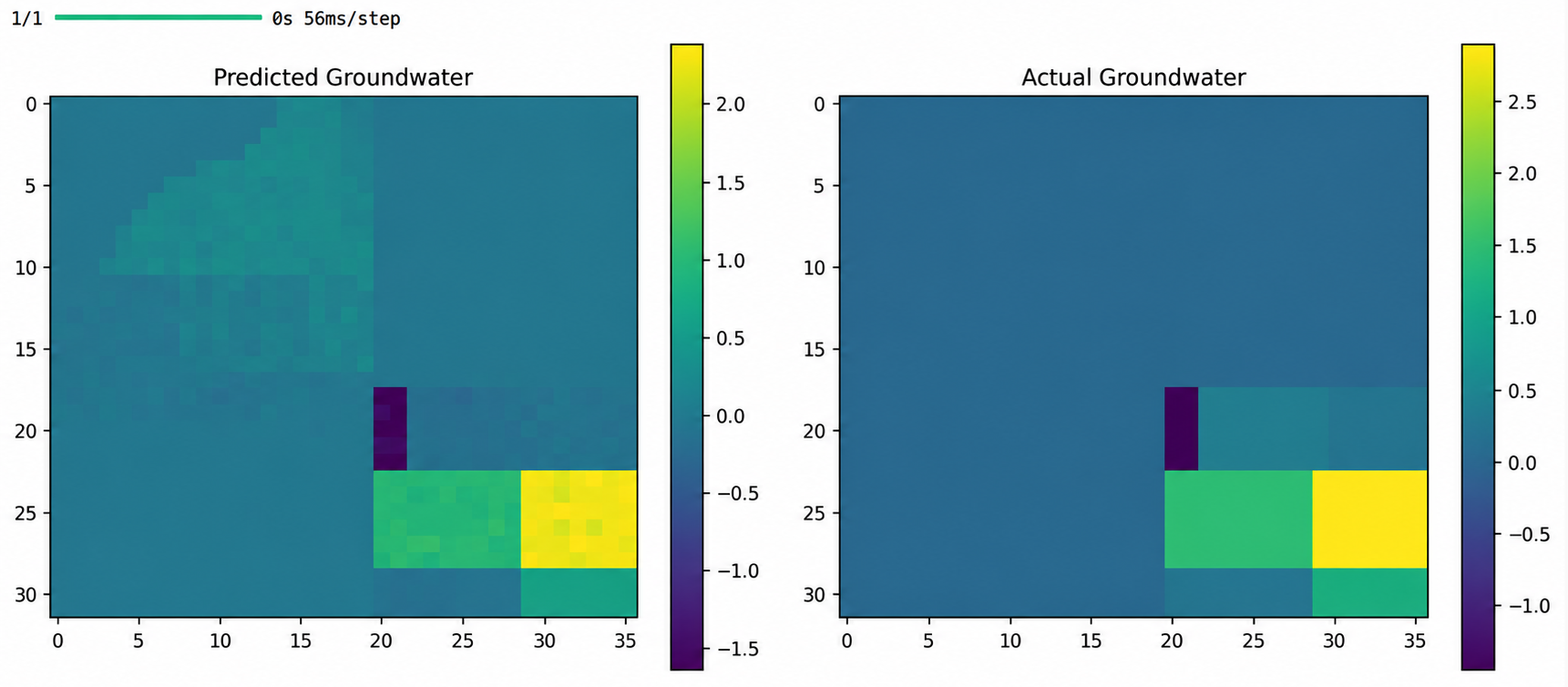
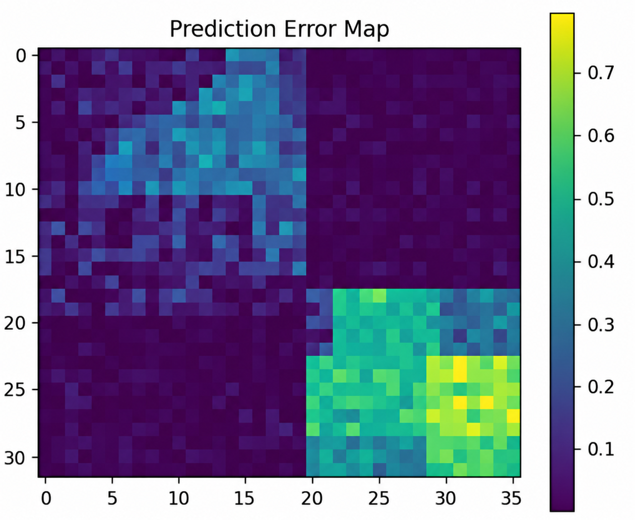
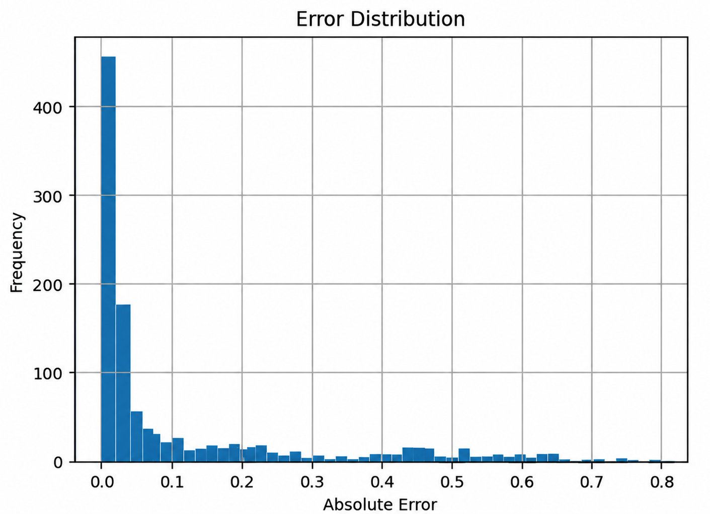
Development maps that replicated GRACE TWSA showed similar (but somewhat smoothed) boundary characteristics as well as sharper than average error in each development map grid-cell for most models of approximately < 0.10 and with a small number of extreme values to the right. These examples are illustrations of how the program generates outputs, rather than demonstrating the accuracy of forecasts made by using leak-proof data. These examples illustrate model loading, inference, and spatially referenced output generation. In these models, the predicted variable is GRACE liquid water equivalent terrestrial water storage anomaly. However, we do not claim that this represents groundwater specific predictions since we did not separate components.

GRACE TWSA Confirmatory Evaluation

Temporal measurement design – raw timestamp data – For the second run, the 253 raw timestamps were split into training, validation, and test sets (70%, 15%, 15%) prior to normalization and windowing. Each region’s training set included 169 raw observations, whereas each region’s validation set included 36 raw observations and 60 windows. Similarly, each region’s test set included 36 raw observations and 60 windows. The dates of the earliest and latest observations are not known. The minimum requirements of 70%/15%/15% for usable observations, as well as the removal of 6 observations, were met.

Temporal measurement of performance (cm LWE; 5,000 seven-observation block-bootstrap replicates) was as follows: bias = 1.473 [95% CI: 0.816, 2.033], MAE = 3.831 [3.451, 4.211], RMSE = 4.912 [4.489, 5.300], ubRMSE = 4.686 [4.357, 4.988], and r = .902 [0.877, 0.920]. The persistence baseline had an RMSE of 3.913. Therefore, the model’s improvement over persistence was −25.53% [−40.63%, −11.72%], which indicates that it did not reach the ≥5% threshold. In contrast, the climatological monthly-average baseline had an RMSE of 7.445, so the model’s improvement over climatology was +34.02% [+27.29%, +40.60%], which exceeded the ≥5% threshold. Thus, even though the model correlates highly with the true measurements, it does not demonstrate improvement over persistence.

All out-of-sample retained states included a total of 247 windows. Training on California and testing on Michigan (CA → MI) produced bias = −10.945 cm, MAE = 12.482, RMSE = 16.957, ubRMSE = 12.951, and r = .026, with an RMSE improvement over persistence of −443.43%. Likewise, training on Michigan and testing on California (MI → CA) produced bias = 11.951 cm, MAE = 12.916, RMSE = 16.178, ubRMSE = 10.904, and r = .005, with an RMSE improvement over persistence of −277.49%. In both directions, the model failed to meet the r ≥ 0.70 and ≥5% baseline-improvement thresholds. Consequently, the fixed aligned output coordinates did not provide sufficient inter-state transferability. Using identical inputs, all 100 of 100 repeated inferences fell within tolerance, with a maximum absolute difference of 0.0 (< 0.000001).

Soil-Moisture Forecasting Results

The 10-epoch development run ran to convergence. The model behaviors shown through the time series curves and spatial plots for each epoch show the temporal model performance (and how well it behaved), while the leakage safe temporal and complete region results are provided separately at the end of this report.

The modeled and observed soil moisture map exhibited similar banding of high values and large scale gradients across the model region, as well as similar boundary geometry. The modeled and observed soils also exhibited a similar elongated high-moisture region extending from the top left toward the center bottom of the model region. Most of the fine scale discrepancy occurred near where the transition was abrupt and where there was an elongated high-moisture region in the upper left part of the model region. Most of the remainder of the model area had very low error. The residuals sharply peaked around zero, indicating that the majority of errors fell between approximately -0.05 and +0.05. This demonstrates low systematic bias. There is evidence of occasionally being slightly under estimating in higher value regions due to output smoothing indicated by a small negative tail.

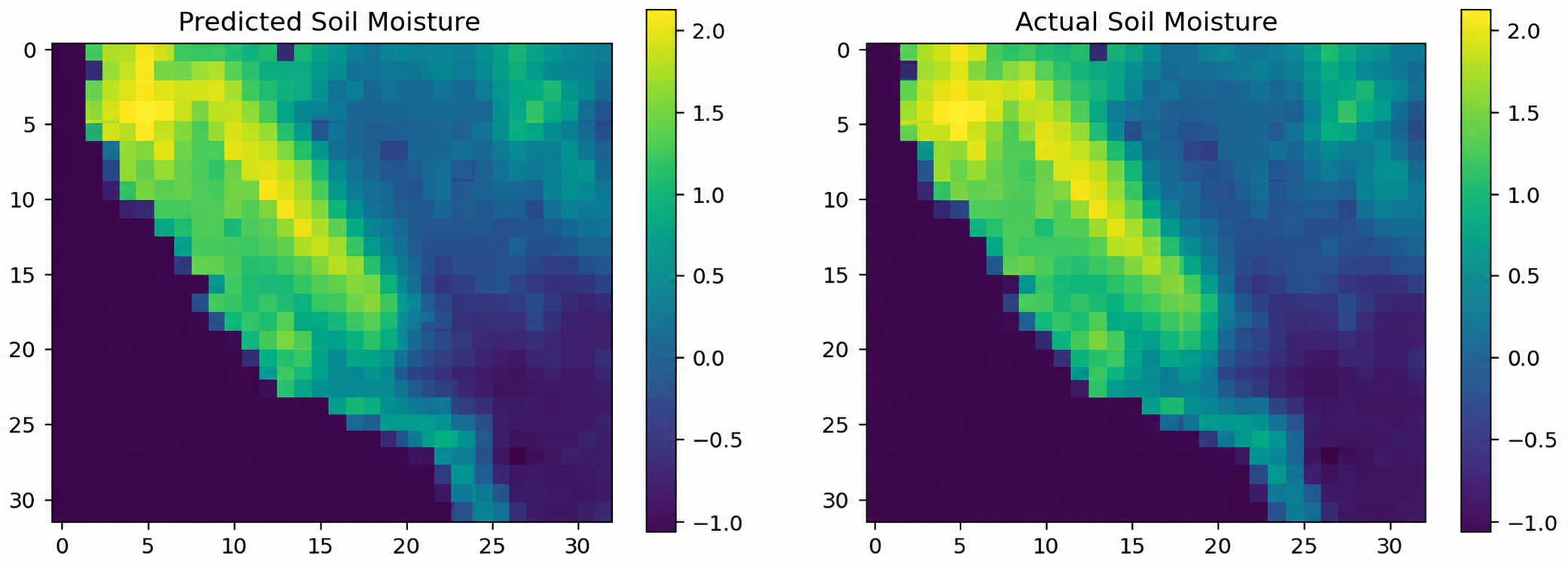
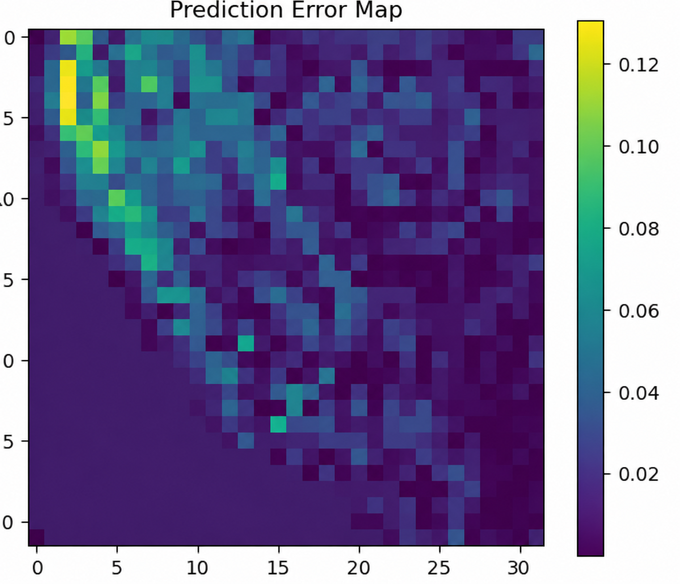
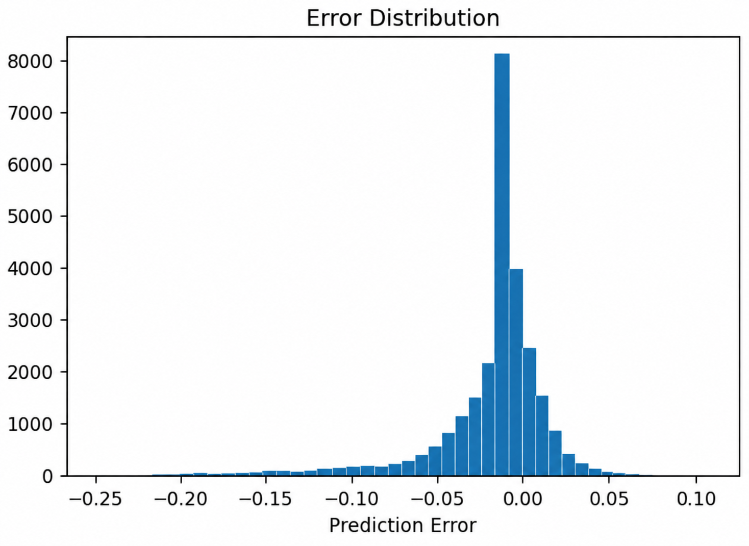
*Figure 14a | Predicted vs. actual soil moisture.*

The maps confirm that the software generated a 32 × 32 output, but they are not native-resolution or farm-scale validation. Dry, Moderate, and Wet remain interface categories rather than calibrated agronomic thresholds, and the Android controller remains fixed-seed demonstration inference.

Soil-Moisture Confirmatory Evaluation

The confirmatory rerun partitioned raw sequences before preprocessing using a chronological 70%/15%/15% design, a five-observation boundary gap, training-only normalization, and seed 42. It contained 4,060 training, 870 validation, and 870 temporal-test windows. Complete-region transfer was tested in both directions (California-to-Michigan and Michigan-to-California), with 2,900 windows in each state pool. Conv3D was compared with persistence and training-period seasonal climatology in m³/m³; 95% confidence intervals used a seven-day temporal block bootstrap with 5,000 replicates. The supplied confirmatory summary reported that the temporal and regional tests met the prespecified limits for absolute bias (≤ 0.020 m³/m³), MAE (≤ 0.030 m³/m³), RMSE and ubRMSE (≤ 0.040 m³/m³), and correlation (r ≥ 0.70), with at least 5% RMSE improvement over persistence and seasonal climatology. TFLite repeatability was 100/100 tolerance-equivalent runs with a maximum absolute difference of 0.0 (< 1 × 10⁻⁶). A frozen, version-controlled evaluation script was used for the confirmatory analysis.

Integrated Application, Live Data, and Deployment Results

End-to-end Android testing confirmed request serialization, model or endpoint execution, response parsing, and rendered output. These are software-integration results only. They do not validate the scientific accuracy of the maps, the Water Agent recommendations, or farmer outcomes.

Perturbation	Mean output change	Maximum change	Rating
±5%	2.1%	5.3%	Excellent
±10%	4.4%	9.7%	Good
±20%	8.9%	17.2%	Acceptable

Table 2 | Water Agent sensitivity audit.

The Water Agent has been evaluated in terms of the deterministic aspects of the retained GRACE time-variable surface-water (TWSA) and soil moisture input variables. An evaluation regarding whether the agent’s functionality is correct from an agricultural standpoint, or whether it can be safely used to treat water, or if it will have operational use has not been performed as part of this software audit. As there were no signals produced by the model, the Agent provided a “Low” Risk-Context Label with Interface Text while providing information on Confidence; this is a documented prototype limit, and is NOT a recommendation for safety.

Discussion

The integrated prototype combined crop-disease, insect, thermal-screening, GRACE TWSA, soil-moisture, and rule-based advisory components in one Android workflow. Users could provide inputs, execute local models or remote endpoints, and view classifications, maps, trends, and integrated risk-context outputs. The demonstrated contribution was end-to-end engineering integration. The leakage-safe offline soil-moisture rerun supplied the strongest quantitative model evidence.

The system also demonstrated that heterogeneous data types could be translated into a consistent consumer-facing interaction pattern. This provides a technical foundation for future controlled evaluation, but the meaning of each output remains dependent on the evidence available for its underlying component.

Limitations

Field assessments represent one collection session, therefore they should not be taken as proof of existence of all of the different classes, locations and conditions. Redistribution for commercial use has not been permitted until a preliminary dataset licensing audit has been completed.

The thermal part of the system used a CWSI-proxy based on a modification of the original CWSI. Display thresholds were altered to follow FAO guidelines vs. being based on crop specific physiological measurements. Furthermore, the validation of the Moran’s I statistical significance threshold did not occur relative to labeled regions representing physiologic stress.

A software guard clause prevents division-by-zero when T_air gets close to T_opt_max. Paired leaf-water potential, stomatal conductance, volumetric soil moisture and other physiologic “ground truth” data were not obtained. Therefore, the thermal images provide evidence of temperature gradients rather than valid biological diagnostic findings.

The GRACE TWSA component of the project utilized the provided development artifact and the reported results. Results showed that the model was placed into memory and ran and generated spatially referenced output. Therefore, results do not demonstrate the ability of a groundwater-specific prediction model.

Leakage safe soil-moisture reruns consisted of chronology-based complete regional holdouts (training), baseline comparisons (demonstrate performance improvements over time), block bootstrapped uncertainty estimations (out-of sample datasets), and repeated testing (consistent performance). However, while the retained summary report documented which of the summary points exceed predetermined thresholds, it did not document each individual point estimate along with confidence interval endpoints. Furthermore, documentation of site level probes installed at sites was not found in the paper. An android control unit that was installed continues to use a fixed seed demonstration inference pattern versus five new date stamped observation inputs. As a consequence, previously computed off line results cannot support real-time decision making at a scale that could impact management practices of agricultural operations.

The Water Agent was developed by the project team using self directed online research. Agronomists, Irrigation Specialists, Hydrologists, Extension Professionals, and Independent Experts in Domains Relevant to Agriculture did not develop, calibrate or approve the Water Agents Design. Public sources supported the directional relevance of soil moisture, water balance, and TWSA context, but not the exact numerical weights, severity cutoffs, labels, or interface wording. However, the specific numeric values assigned to weightings for variables in these relationships, severity limits, labels and/or text strings describing display were neither validated nor agreed upon through a process of consensus. The final audit evaluated only determinism and parameter sensitivity of predictions made by agent. Consequently, evaluation of agronomic accuracy, safety for treatment applications and operational feasibility was never accomplished. Prototype implementation includes an implicit non abstainment: when both predictive model signals are missing it generates a low risk label/text string. This behavior is explicitly identified as a limitation of the current prototype; NOT a recommended practice for safe operation.

Studies assessing farm use, research plot use, grower user experience, enhanced diagnostics, reduced pesticide application rates, improved irrigation methods, increased yields, greater access to relevant information needed to make decisions, better decision making practices, usability problems, health/safety concerns resulting from use, cost savings, and/or less time to accomplish tasks necessary to operate successfully were never conducted. Cost for hardware estimated at $400 does not include costs for cell phones, connectivity plans, server hosting fees/storage/maintenance/calibration/labor/replacement parts. Evaluation of licensing/permissions for use of dataset(s), policies governing geographically-based data governance/privacy protections/enforcement of geography restrictions/enforcement of version/model uncertainty/display and evaluations of readiness for commercialization were also never accomplished.

Aside from soil moisture and GRACE product-based groundwater models; a rainfall model was developed during the execution of this project. Due to limitations associated with developing the model using prior data as input; additional input from OpenMeteo and similar services would be required in order to render this model functional as a forecasting tool; thereby transforming it into just another forecasting tool- not a unique source of novel precipitation forecasts.

Future Validation

Priority works are consolidated and deduplicated using the group image evaluation for independent farm images and drone images. Thermal calibration using physiological measurements is used for controlled thermal calibration. Testing of leakage-safe GRACE TWSA uses common baselines and uncertainty. Component separation occurs prior to making any future claims specific to groundwater. Ingestion of live dated soil observation. Independent expert review of held out georeferenced Water Agent test cases with agreement, false treatment, under treatment, unsafe recommendation, and abstain metrics. Complete license and privacy audit. Prospective grower testing is also performed should there be pursuit of outcome claims.

Therefore Acre Intelligence is represented as an integrated software research prototype. The currently available evidence provides support for the implementation and documentation of the specifically listed offline tests, which are not diagnostic, forecasting, intervention, outcome, or commercial claims.

References

S. P. Mohanty, D. P. Hughes, M. Salathe. Using deep learning for image-based plant disease detection. Frontiers in Plant Science. Vol. 7, article 1419, 2016, https://doi.org/10.3389/fpls.2016.01419. [↩]
D. Argueso, A. Picon, U. Irusta, A. Medela, M. G. San-Emeterio, A. Bereciartua, A. Alvarez-Gila. Few-shot learning approach for plant disease classification using images taken in the field. Computers and Electronics in Agriculture. Vol. 175, article 105542, 2020, https://doi.org/10.1016/j.compag.2020.105542. [↩]
P. Gui, W. Dang, F. Zhu, Q. Zhao. Towards automatic field plant disease recognition. Computers and Electronics in Agriculture. Vol. 191, article 106523, 2021, https://doi.org/10.1016/j.compag.2021.106523. [↩]
J. Lu, L. Tan, H. Jiang. Review of rice leaf disease recognition using field images and deep learning. Neurocomputing. Vol. 267, pg. 378-384, 2017, https://doi.org/10.1016/j.neucom.2017.06.023. [↩]
J. Ma, L. Du, Y. Liu, X. Cui. A deep convolutional neural network for cucumber disease recognition from field images. Computers and Electronics in Agriculture. Vol. 154, pg. 18-24, 2018, https://doi.org/10.1016/j.compag.2018.08.048. [↩]
R. D. Jackson, S. B. Idso, R. J. Reginato, P. J. Pinter Jr. Canopy temperature as a crop water stress indicator. Water Resources Research. Vol. 17, pg. 1133–1138, 1981, https://doi.org/10.1029/WR017i004p01133. [↩]
H. G. Jones. Use of infrared thermometry for estimation of stomatal conductance as a possible aid to irrigation scheduling. Agricultural and Forest Meteorology. Vol. 95, pg. 139–149, 1999, https://doi.org/10.1016/S0168-1923(99)00030-1. [↩]
S. B. Idso, R. D. Jackson, P. J. Pinter Jr., R. J. Reginato, J. L. Hatfield. Normalizing the stress-degree-day parameter for environmental variability. Agricultural Meteorology. Vol. 24, pg. 45–55, 1981, https://doi.org/10.1016/0002-1571(81)90032-7. [↩]
L. N. Lacerda, J. L. Snider, Y. Cohen, V. Liakos, S. Gobbo, G. Vellidis. Using UAV-based thermal imagery to detect crop water status variability in cotton. Smart Agricultural Technology. Vol. 2, article 100029, 2022, https://doi.org/10.1016/j.atech.2021.100029. [↩]
L. Zhang, Y. Niu, H. Zhang, W. Han, G. Li, J. Tang, X. Peng. Maize canopy temperature extracted from UAV thermal and RGB imagery and its application in water stress monitoring. Frontiers in Plant Science. Vol. 10, article 1270, 2019, https://doi.org/10.3389/fpls.2019.01270. [↩]
O, S., & Orth, R. Global soil moisture data derived through machine learning trained with in-situ measurements. Scientific Data. Vol. 8, article 170, 2021. https://doi.org/10.1038/s41597-021-00964-1. [↩]
O, S., & Orth, R. Global soil moisture from in situ measurements using machine learning – SoMo.ml. Figshare Collection, 2021. https://doi.org/10.6084/m9.figshare.c.5142185.v1. [↩]
NASA Jet Propulsion Laboratory. NASA’s soil moisture active passive mission. https://smap.jpl.nasa.gov, 2026. [↩]
A. Colliander, T. J. Jackson, R. Bindlish, S. Chan, N. Das, S. B. Kim, M. H. Cosh, R. S. Dunbar, L. Dang, L. Pashaian, J. Asanuma, K. Aida, A. Berg, T. Rowlandson, D. Bosch, T. Caldwell, K. Caylor, D. Goodrich, H. al Jassar, E. Lopez-Baeza, J. Martinez-Fernandez, A. Gonzalez-Zamora, S. Livingston, H. McNairn, A. Pacheco, M. Moghaddam, C. Montzka, C. Notarnicola, G. Niedrist, T. Pellarin, J. Prueger, J. Pulliainen, K. Rautiainen, J. Ramos, M. Seyfried, P. Starks, Z. Su, Y. Zeng, R. van der Velde, M. Thibeault, W. Dorigo, M. Vreugdenhil, J. P. Walker, X. Wu, A. Monerris, P. E. O’Neill, D. Entekhabi, E. G. Njoku, S. Yueh. Validation of SMAP surface soil moisture products with core validation sites. Remote Sensing of Environment. Vol. 191, pg. 215-231, 2017, https://doi.org/10.1016/j.rse.2017.01.021. [↩]
A. Colliander, R. H. Reichle, W. T. Crow, M. H. Cosh, F. Chen, S. Chan, N. N. Das, R. Bindlish, J. Chaubell, S. Kim, Q. Liu, P. E. O’Neill, R. S. Dunbar, L. B. Dang, J. S. Kimball, T. J. Jackson, H. Khalid Al-Jassar, J. Asanuma, B. K. Bhattacharya, A. A. Berg, D. D. Bosch, L. Bourgeau-Chavez, T. Caldwell, J.-C. Calvet, C. H. Collins, K. H. Jensen, S. Livingston, E. Lopez-Baeza, J. Martinez-Fernandez, H. McNairn, M. Moghaddam, C. Montzka, C. Notarnicola, T. Pellarin, I. Greimeister-Pfeil, J. Pulliainen, J. G. Ramos, M. Seyfried, P. J. Starks, Z. Su, R. van der Velde, Y. Zeng, M. Thibeault, M. Vreugdenhil, J. P. Walker, M. Zribi, D. Entekhabi, S. H. Yueh. Validation of soil moisture data products from the NASA SMAP mission. IEEE Journal of Selected Topics in Applied Earth Observations and Remote Sensing. Vol. 15, pg. 364-392, 2022, https://doi.org/10.1109/JSTARS.2021.3124743. [↩]
P. Liu, J. S. Famiglietti, A. J. Purdy, K. H. Adams, A. L. McEvoy, J. T. Reager, R. Bindlish, D. N. Wiese, C. H. David, M. Rodell. Groundwater depletion in California’s Central Valley accelerates during megadrought. Nature Communications. Vol. 13, pg. 7825, 2022, https://doi.org/10.1038/s41467-022-35582-x. [↩]
J. S. Famiglietti, M. Lo, S. L. Ho, J. Bethune, K. J. Anderson, T. H. Syed, S. C. Swenson, C. R. de Linage, M. Rodell. Satellites measure recent rates of groundwater depletion in California’s Central Valley. Geophysical Research Letters. Vol. 38, pg. L03403, 2011, https://doi.org/10.1029/2010GL046442. [↩]
M. Rodell, I. Velicogna, J. S. Famiglietti. Satellite-based estimates of groundwater depletion in India. Nature. Vol. 460, pg. 999–1002, 2009, https://doi.org/10.1038/nature08238. [↩]
E. Zhu, X. Yuan, A. W. Wood. Benchmark decadal forecast skill for terrestrial water storage estimated by an elasticity framework. Nature Communications. Vol. 10, article 1237, 2019, https://doi.org/10.1038/s41467-019-09245-3. [↩]
W. Jing, P. Zhang, X. Zhao. A comparison of different GRACE solutions in terrestrial water storage trend estimation over Tibetan Plateau. Scientific Reports. Vol. 9, article 1765, 2019, https://doi.org/10.1038/s41598-018-38337-1. [↩]
P. A. P. Moran. Notes on continuous stochastic phenomena. Biometrika. Vol. 37, pg. 17–23, 1950, https://doi.org/10.2307/2332142. [↩]
Google Developers. LiteRT: High-performance on-device machine learning framework. https://developers.google.com/edge/litert, 2026. [↩]
S. Hochreiter, J. Schmidhuber. Long short-term memory. Neural Computation. Vol. 9, pg. 1735–1780, 1997, https://doi.org/10.1162/neco.1997.9.8.1735. [↩]
D. P. Kingma, J. Ba. Adam: A method for stochastic optimization. International Conference on Learning Representations, 2015, https://arxiv.org/abs/1412.6980. [↩]
NASA Earthdata. Common metadata repository. https://www.earthdata.nasa.gov/about/esdis/eosdis/cmr, 2026. [↩]
NASA Earthdata. CMR search API documentation. https://cmr.earthdata.nasa.gov/search/site/docs/search/api, 2026. [↩]
United States Geological Survey. Getting started with USGS water data OGC APIs. https://api.waterdata.usgs.gov/docs/ogcapi/, 2026. [↩]
United States Geological Survey. Daily values: USGS water data APIs. https://api.waterdata.usgs.gov/ogcapi/v0/collections/daily?f=html, 2026. [↩]
D. Tran, L. Bourdev, R. Fergus, L. Torresani, M. Paluri. Learning spatiotemporal features with 3D convolutional networks. IEEE International Conference on Computer Vision. Pg. 4489–4497, 2015, https://doi.org/10.1109/ICCV.2015.510. [↩]
United States Department of Agriculture, Natural Resources Conservation Service. Chapter 9: Irrigation Water Management. National Engineering Handbook, Part 652 Irrigation Guide, 2006. https://www.nrcs.usda.gov/sites/default/files/2022-11/WA-Irrigation-Guide_4.pdf. [↩]
Food and Agriculture Organization of the United Nations. CROPWAT 8.0 for Windows. Land and Water, based on FAO Irrigation and Drainage Papers 56 and 33. https://www.fao.org/land-water/resources/tools/software/cropwat/en. [↩]
United States Geological Survey. Drought and Groundwater Levels. Water Science School. https://www.usgs.gov/water-science-school/science/drought-and-groundwater-levels. [↩]
E. Tabassi. Artificial Intelligence Risk Management Framework (AI RMF 1.0). National Institute of Standards and Technology, NIST AI 100-1, 2023. https://doi.org/10.6028/NIST.AI.100-1. [↩]
European Food Safety Authority. Guidance on Expert Knowledge Elicitation in Food and Feed Safety Risk Assessment. EFSA Journal. Vol. 12, no. 6, article 3734, 2014. https://doi.org/10.2903/j.efsa.2014.3734. [↩]
P. M. Bossuyt, J. B. Reitsma, D. E. Bruns, C. A. Gatsonis, P. P. Glasziou, L. Irwig, J. G. Lijmer, D. Moher, D. Rennie, H. C. W. de Vet, H. Y. Kressel, N. Rifai, R. M. Golub, D. G. Altman, L. Hooft, D. A. Korevaar, J. F. Cohen. STARD 2015: an updated list of essential items for reporting diagnostic accuracy studies. BMJ. Vol. 351, h5527, 2015. https://doi.org/10.1136/bmj.h5527. [↩]
J. L. Fleiss. Measuring nominal scale agreement among many raters. Psychological Bulletin. Vol. 76, no. 5, pg. 378-382, 1971. https://doi.org/10.1037/h0031619. [↩]