Stochastic Biomass Forecasting of Golden Tilefish Using the Deep Galerkin Method

Abstract

Accurate biomass forecasting is important for sustainable fisheries management where population dynamics are influenced by environmental variability. In this study, a biomass model is developed for Golden Tilefish (Lopholatilus chamaeleonticeps) using a stochastic Gompertz growth model with multiplicative environmental noise.  Biomass forecasts were generated through Monte Carlo simulation. The Deep Galerkin Method (DGM), a neural network–based mesh-free PDE solver, was used to approximate a complementary value function to represent expected discounted management risk associated with biomass declining below a specified management threshold. The stochastic Gompertz model was initialized using the NOAA-reported 2019 biomass estimate and projected forward under a single calibrated parameter set and year-specific harvest assumptions. A final ensemble of 1,000 stochastic trajectories was evaluated against NOAA-reported biomass estimates for 2020–2023. The ensemble-median forecast produced a mean absolute error (MAE) of 433,676 lbs, a root mean squared error (RMSE) of 540,360 lbs, and a mean bias of −1,297 lbs, with all observed biomass estimates falling within the corresponding 10th–90th percentile prediction intervals. The stochastic model produced substantially lower forecast error than the naive persistence baseline. It modestly improved point-forecast performance relative to the deterministic Gompertz formulation, for which RMSE was nearly identical. These results demonstrate the utility of stochastic biomass modeling for representing forecast uncertainty while illustrating how DGM-based value functions can provide complementary information concerning management-threshold risk. The combined framework provides a basis for evaluating both expected biomass dynamics and uncertainty which is relevant to risk-aware fisheries management.

Keywords: Stochastic Biomass Modeling, Golden Tilefish, Deep Galerkin Method, Monte Carlo Simulation, Fisheries Stock Forecasting, Uncertainty Quantification

Abbreviations

ACL — Annual Catch Limit
DGM — Deep Galerkin Method
MAE — Mean Absolute Error
MAPE — Mean Absolute Percentage Error
MSST — Minimum Stock Size Threshold
NOAA — National Oceanic and Atmospheric Administration
ODE — Ordinary Differential Equation
PDE — Partial Differential Equation
PI — Prediction Interval
RMSE — Root Mean Squared Error
SDE — Stochastic Differential Equation
SPDE — Stochastic Partial Differential Equation

Introduction

Deterministic models of fishery stocks have often fall short due to their inability to account for unpredictable ecological systems¹. This limitation can lead to inaccurate management decisions that affect the sustainability of fishery resources². Deterministic frameworks typically rely on smooth and average trends, overlooking random fluctuations from environmental factors such as sudden ocean temperature changes and changing fishing pressures. Biomass-dynamic models may also be affected changes in stock productivity over time. This is why it is important to consider nonstationary biological factors when interpreting population trajectories³. Without considering such changes and factors, forecasts for complex ecosystems such as those supporting Golden Tilefish can become less reliable and prone to systematic biases.

The Golden Tilefish (Lopholatilus chamaeleonticeps) is important in U.S. fisheries, both ecologically and economically, and serves as a focal species in this study.  It exemplifies the challenges of forecasting populations in ecosystems subject to environmental uncertainty. Accounting for environmental uncertainty has become increasingly important for fisheries management since climate-driven changes can alter future biomass and catch trajectories and may reduce the effectiveness of management strategies if they do not account for changing ecosystem conditions⁴. Recent fisheries-management frameworks have emphasized incorporating climate-driven changes in stock productivity and distribution explicitly into their assessment and management processes⁵. Incorporating stochasticity into population models becomes essential to account for variability and uncertainty. Simulation-based evaluations of fisheries rebuilding strategies have demonstrated that management performance can depend strongly on how uncertainty is represented and incorporated into harvest-control decisions⁶. Carpenter et al. emphasized that disregarding stochastic elements can amplify management risks^7,8, elevating the probability of resource collapse and undermining conservation efforts. SPDEs offer a mathematic framework for introducing randomness into dynamic system models. This allows predictions to more closely match with ecological fluctuations.

In theory, SPDEs offer fidelity. However, solving them efficiently is a computational challenge. This is especially true in high-dimensional or nonlinear systems⁹. Deep-learning approaches are an alternative for approximating high-dimensional PDE solutions¹⁰, and work by extending physics-informed neural-network approaches to time-dependent stochastic PDEs and uncertainty propagation¹¹.  Physics-informed neural-networks have demonstrated the ability for deep learning models to solve forward and inverse differential-equation problems, including stochastic PDEs¹². The DGM addresses the computational challenge by using neural networks to approximate PDE solutions without requiring discretization gridsgrids¹³. In contrast to numerical solvers, DGM learns the solution function by minimizing the PDE residuals over randomly sampled points. Ecological systems are irregular, noisy, and often lack robust observational datasets.  

This study uses a stochastic differential equation (SDE) coupled with a DGM-based PDE framework to evaluate a population model for Golden Tilefish biomass forecasting.  We propose a methodology for representing both biomass uncertainty and management-related risk. We do this by combining stochastic biomass dynamics with a DGM-based approximation of the associated threshold-risk value function.  Recent advances in marine forecasting have shown that biologically relevant changes in fish habitat and distribution can be predicted more reliably over several years, demonstrating the value of forecasting for marine resource management¹⁴. Current marine management tools incorporate ecological forecasts to provide information during climate extremes and demonstrate how such forecasts can support resource-management decisions¹⁵.  Our goal is to improve management of fisheries by providing robust biomass estimates that better reflect ecological realities.  This will ultimately lead to more sustainable resource exploitation.

Management Definitions

Three different management-related quantities are used in this study. 1) The Annual Catch Limit (ACL) is a regulatory limit on allowable catch. 2) Commercial landings represent the realized removals reported for the fishery. 3) The threshold parameter K, which defines a model-based biomass trigger used to quantify the penalty associated with biopmass declining below a specified threshold level. The biomass forecasting simulations in this study do not use the ACL as a fixed harvest term; instead, they incorporate year-specific Mid-Atlantic/Southern New England commercial landings. K appears in the DGM value function and is treated as a management-risk threshold and not treated as an independently estimated biological reference point.

Methods

Mathematical Model

Stochastic Biomass Dynamics

Fish populations are influenced by density-dependent biological processes and stochastic drivers such as environmental variability, fishing pressure, and recruitment fluctuations. To model these, we consider a stochastic version of the Gompertz growth model, a formulation that has been extensively utilized to describe bounded growth in ecological systems, including fish populations¹⁶.

We consider a stochastic process representing fish biomass at time , governed by the following stochastic differential equation:

where denotes the carrying capacity of the system, is the intrinsic rate of mean reversion toward this carrying capacity, quantifies the magnitude of stochastic environmental fluctuations, and is a standard Brownian motion.

In the forecasting simulations presented in this study, the parameter a was not fixed a priori as an independently established biological carrying capacity. Instead, it was estimated jointly with the mean-reversion parameter b, environmental stochasticity parameter , and harvest-scaling factor during model calibration. The final calibrated value was million lbs. Accordingly, a is interpreted here as the asymptotic biomass level of the fitted Gompertz dynamics under the available biomass and harvest data rather than as a direct estimate of the maximum biological carrying capacity of the Golden Tilefish stock.

The drift term 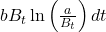allows the system to exhibit density-dependent feedback, and causes biomass growth to decelerate as it nears carrying capacity. This logarithmic feedback works well for species like Golden Tilefish, where growth saturation occurs gradually due to resource competition, habitat constraints, and ecological regulation mechanisms.

The diffusion term introduces multiplicative environmental noise, accounting for the observation that larger populations experience proportionally larger absolute fluctuations. This modeling choice accounts for external factors which are unpredictable, such as recruitment variability, temperature anomalies, and episodic fishing pressures. This ensures that variability scales with the magnitude of biomass. The use of multiplicative noise, as opposed to additive formulations, captures the heteroscedastic nature of ecological systems, where variance is state-dependent.

Derivation of Associated PDE

We define a value function as the expected discounted management risk associated with biomass falling below a critical threshold in order to analyze the effect of biomass depletion under uncertain conditions. In the context of Golden Tilefish, provides a continuous measure of the expected cost of stock depletion and the need to intervene. Rather than representing a financial quantity, the value function quantifies ecological risk throughout the biomass-time domain and provides information beyond point estimates of future biomass. Applying It Lemma to , we obtain the second-order linear PDE governing temporal evolution:

This PDE describes deterministic growth dynamics, stochastic fluctuations, and temporal discounting. This captures how uncertainty propagates through time and space. Unlike deterministic ordinary differential equations (ODEs), this allows calculation of outcomes under stochastic influences. PDE-based formulations are powerful because they provide information about management risk and threshold behavior throughout the biomass-time domain. In the present study, Monte Carlo simulation is used to generate biomass trajectories, while the PDE framework quantifies threshold-related risk.

The derived PDE resembles those found in financial option pricing theory, where asset values evolve stochastically, and derivative payoffs depend on reaching certain boundaries. We exploit this in the boundary-condition formulation.

Boundary Conditions

We pose an inequality-constrained PDE inspired by the mathematical structure of American-style option pricing, to incorporate adaptive management triggers¹⁷. The terminal payoff condition is given by:

where K denotes the biomass threshold used in the management-risk value function. In the implemented DGM formulation, K was set to 315,484 lbs and serves as a model-defined trigger below which the terminal payoff becomes positive. The terminal payoff therefore increases as biomass falls farther below the specified threshold. This threshold should be interpreted as a modeling parameter used to illustrate the management-risk framework rather than as the regulatory Annual Catch Limit or an independently estimated Minimum Stock Size Threshold. The biomass forecasting simulations themselves do not use K to determine harvest removals; harvest pressure is represented separately using year-specific reported commercial landings.

The inequality-constrained formulation is inspired by the mathematical structure of American-style option problems, in which a continuation value is compared with an immediate payoff. In the present ecological interpretation, the payoff max (K−B,0) represents a penalty associated with biomass falling below the specified model threshold. The DGM approximation is constrained so that the value function does not fall below this payoff while satisfying the governing PDE in the continuation region. This provides a mathematical framework for representing threshold-related management risk under stochastic biomass dynamics and is consistent with previous work demonstrating the importance of environmental stochasticity in fisheries management and harvest decision-making¹⁸.  

By formulating the problem this way, the model provides a continuous representation of the penalty associated with biomass states below the specified threshold, complementing the biomass forecasts with information about threshold-related management risk.

In this study, the threshold parameter K is therefore interpreted as a model-defined biomass trigger rather than as an independently established MSST. Biomass values below K generate a positive depletion penalty, with the magnitude of the terminal payoff increasing as biomass declines farther below the threshold. The American-option analogy provides the mathematical structure for this threshold-dependent value function; however, the present analysis does not estimate or validate an optimal fisheries intervention rule or intervention timing. Accordingly, the DGM results are interpreted as a complementary representation of threshold-related risk rather than as a direct prescription for management action.

Deep Galerkin Implementation

Deep Galerkin Method

To approximate the solution , we adopt the DGM introduced by Sirignano and Spiliopoulos, a mesh-free neural network framework designed to solve PDEs by minimizing their residuals at randomly sampled domain points¹³. DGM circumvents the computational challenges of grid-based solvers by using the universal function approximation capacity of deep networks. The training objective is formulated as a composite loss function that enforces the PDE operator, boundary constraints, and terminal conditions across the solution domain.

DGM Network Architecture

The Deep Galerkin Method architecture employed in this study follows the method introduced by Sirignano and Spiliopoulos (2018), using a fully connected neural network with residual information flow between layers. Temporal and spatial inputs are supplied simultaneously to the network, allowing the solution to be approximated over the continuous time-biomass domain without explicit discretization. Unlike recurrent neural network architectures such as GRUs or LSTMs, the implemented DGM network propagates information through skip connections and nonlinear transformations, which provide sufficient expressive capacity for the time-dependent PDE considered in this work. To improve numerical stability, the inputs were normalized according to

where T denotes the terminal time and is the asymptotic biomass parameter used in the DGM PDE calculation. The network output represents the value function associated with biomass risk and management thresholds and is parameterized by the trainable weights of the DGM architecture.

Loss Function Design

The loss function used to train the network incorporates the interior PDE residual,the inequality constraint associated with the threshold-dependent payoff, and terminal payoff conditions at . The total loss is expressed as:

Automatic differentiation is used to compute the gradient terms. To maintain differentiability during training, the inequality constraint is enforced using a soft ReLU barrier function. Terminal conditions are explicitly imposed by sampling boundary points at and minimizing the deviation from the prescribed payoff.

Sampling and Training Strategy

The network is trained using the Adam optimizer with a fixed learning rate of . The DGM solution domain extended from approximately 0 to 1 year in time, while biomass samples were drawn from approximately 0 to 946,452 lbs. At each sampling stage, 1,000 interior domain points were resampled from this domain, together with 100 terminal-boundary samples . Each sampling stage comprises 10 Adam optimization steps and also minimizes the total loss function iteratively. Given the importance of the threshold region (where BK), sampling is adaptively biased toward this domain to enhance model accuracy near the critical threshold. The PDE differential operator imposed empirical convergence and smoothness requirements in the selection of hyperparameters. These included layer count (3 layers), nodes per layer (50), and activation functions (tanh). The distribution of collocation points can materially affect the performance of neural PDE solvers, and recent work has demonstrated that adaptive sampling strategies can improve accuracy by concentrating training points in regions characterized by larger residual error¹⁹.

Training, Reproducibility, and Convergence

DGM training was performed for a fixed computational budget of 500 sampling stages, with 10 optimization steps per stage, corresponding to 5,000 optimization steps per training run. No loss-based early-stopping criterion was applied. To assess sensitivity to random initialization and domain sampling, DGM training was repeated using five random seeds (42–46). During this procedure the model architecture, training configuration, and PDE parameters remained fixed. Across these runs, the final total loss was (2.28±0.30)×1010 (mean ± SD), with individual final losses ranging from 1.96×1010 to 2.66×1010. These repeated runs indicate that the final composite loss remained within the same order of magnitude across random initializations and stochastic domain samples. Training was performed on a Windows 11 workstation equipped with an AMD Ryzen 7 7800X3D 8-Core Processor. The TensorFlow 1.15 environment recognized only the CPU device. No GPU acceleration was used. Across the five repeated training runs, mean runtime was 124.14 ± 9.03 seconds (approximately 2.07 minutes per run). Repeated-run diagnostics are particularly relevant for neural PDE solvers because optimization of composite physics-informed loss functions can exhibit training difficulties associated with imbalanced gradients among loss components²⁰.

Implementation Details

The DGM was implemented using TensorFlow 1.15, and the Adam optimizer was used to perform network optimization. The architecture was formed by three fully connected hidden layers, each with 50 neurons with each layer receiving concatenated temporal and spatial inputs. Skip connections within the DGM modules facilitated information propagation through the network. The principal forecasting parameters, simulation settings, and DGM configuration used in the final analysis are summarized in Table 1.

Symbol/quantity	Final value	Units	Source/estimation method
	11.4375 million	lbs biomass	Calibrated jointly against NOAA biomass observations
	0.26875	year-1	Calibrated jointly against NOAA biomass observations
	0.080	year-1/2	Calibrated environmental stochasticity parameter
Harvest-scaling factor	0.105	dimensionless	Calibrated coefficient applied to reported Mid-Atlantic/Southern New England commercial landings
Initial biomass	8.53 million	Lbs biomass	NOAA-reported 2019 biomass estimate
Simulation timestep	1/12	year	Monthly simulation interval
Ensemble size	1,000	trajectories	Final Monte Carlo ensemble
Random seed	42	—	Fixed for reproducibility
DGM hidden layers	3	layers	Model configuration
Nodes per hidden layer	50	nodes	Model configuration
Learning rate	0.001	—	Adam optimizer setting
Interior samples	1,000	points/stage	DGM training configuration
Terminal samples	100	points/stage	DGM training configuration
Sampling stages	500	stages	DGM training configuration
Optimization steps	10	steps/stage	DGM training configuration
Management-risk threshold K	315,484	lbs biomass	Model-defined threshold used in DGM value function
DGM time domain	0-1	years	Computational PDE domain
DGM biomass sampling domain	0-946,452	lbs biomass	Computational PDE sampling domain; upper sampling bound
DGM asymptotic biomass parameter	1.5 million	lbs biomass	Parameter used in DGM PDE training
DGM mean-reversion parameter	0.25	year-1	Parameter used in DGM PDE training
DGM stochasticity parameter	0.50	year-1/2	Parameter used in DGM PDE training
Discount rate	0.05	year-1	DGM value-function parameter

The DGM value-function calculation and the Monte Carlo biomass forecast use distinct parameterizations because they serve different purposes in the present framework. The DGM parameters define the computational PDE problem used to illustrate threshold-related management risk, whereas the calibrated stochastic Gompertz parameters are used to generate and evaluate the biomass forecasts.

The stochastic Gompertz parameters used for biomass forecasting were calibrated against NOAA-reported Golden Tilefish biomass observations. Rather than prescribing the carrying-capacity parameter (a), the mean-reversion parameter (b), environmental stochasticity (), and a harvest-scaling factor were jointly evaluated over predefined parameter ranges. Candidate parameter combinations were assessed using Monte Carlo ensembles, with model fit evaluated from the median simulated biomass at the annual observation points. The calibration objective incorporated root mean squared error (RMSE), absolute bias, and maximum absolute annual error to discourage parameter combinations that achieved a low average error at the expense of a large error in an individual year.

The selected parameter combination was a=11.4375 million lbs, b=0.26875, =0.080, and a harvest-scaling factor of 0.105. Harvest pressure was represented using annual commercial Golden Tilefish landings corresponding to the Mid-Atlantic/Southern New England stock and not a constant removal term. Annual landings were expressed in live-weight pounds and divided by 12.  It was applied as monthly harvest inputs after multiplication by the calibrated harvest-scaling factor. At each monthly simulation step, the scaled harvest input was subtracted from the preceding biomass before application of the Gompertz growth update and stochastic environmental term. The harvest-scaling factor is a calibrated coefficient controlling how reported landings enter the discrete biomass process. It should not be interpreted as the proportion of reported harvest that actually occurred. It allows harvest pressure to vary among years at the same time maintaining the monthly temporal resolution of the stochastic simulation. The calibrated value of a should therefore be interpreted as the effective long-run biomass level implied by the fitted stochastic Gompertz model under the available biomass and harvest data, rather than as an independently established biological estimate of maximum stock biomass.

Training was conducted over 500 sampling stages. Fresh domain samples were drawn at each stage to ensure adequate exploration of the solution space. Automatic differentiation was utilized to compute gradient terms required for the PDE residual and a soft ReLU penalty was applied to the inequality constraint region to maintain adherence to the inequality constraint in a differentiable manner.

Biomass trajectories were generated through Monte Carlo simulation of the stochastic Gompertz process at monthly intervals ( year). Environmental stochasticity was represented using the calibrated value , with Gaussian innovations sampled from a standard normal distribution and scaled by the square root of the monthly timestep. Harvest pressure was based on reported annual Golden Tilefish landings, with each annual value divided by 12 to obtain a monthly removal and multiplied by the calibrated harvest-scaling factor of 0.105. The final reported forecast used an ensemble of 1,000 stochastic trajectories with NumPy random seed 42 to permit reproducible generation of the reported ensemble statistics and prediction intervals.

A one-at-a-time sensitivity analysis was used to evaluate the robustness of the stochastic biomass forecasts to uncertainty in the calibrated model parameters. The asymptotic biomass parameter a, mean-reversion parameter b, environmental stochasticity parameter σ, and harvest-scaling coefficient were each varied independently by from their calibrated baseline values. All other parameters were held fixed. A 1,000-member Monte Carlo ensemble was used to evaluate each scenario. In order to isolate the effect of parameter perturbation from Monte Carlo sampling variability, the same random seed and corresponding stochastic draws were used across scenarios. Sensitivity was evaluated using MAE, RMSE, mean bias, MAPE, and the mean width of the 10th–90th percentile prediction interval over the 2020–2023 evaluation period. The evaluation of parameter sensitivity and ensemble behavior is consistent with broader stock-assessment approaches that use ensembles to characterize uncertainty in biological parameters and resulting management quantities²¹.

In calibrating the model, the 2019 NOAA biomass estimate was used as the initial condition and the 2020–2023 biomass observations were used as calibration targets²². Candidate parameter combinations were evaluated according to their ability to reproduce these annual observations while maintaining stochastic ensemble behavior. After selection of the final parameter set, biomass trajectories were generated forward from the 2019 initial condition under the fixed calibrated parameters and year-specific harvest assumptions. Thus, individual simulated trajectories were not adjusted to match each subsequent NOAA observation; rather, the historical observations were used collectively to select the model parameters before the final ensemble simulation. This approach allows the resulting trajectories and prediction intervals to reflect stochastic variability under a single calibrated model rather than year-by-year resetting of the biomass state.

Relationship Between DGM and Biomass Forecasting

Although the Deep Galerkin Method was used to approximate the value function V(t,B) associated with the stochastic control formulation, the biomass forecasts presented in this study were generated independently through Monte Carlo simulation of the stochastic Gompertz process. The DGM output therefore serves primarily as a management-oriented quantity rather than as the direct forecasting engine. Accordingly, the DGM solution is not used to generate the biomass trajectories shown in the forecast figures; instead, it provides a separate threshold-risk quantity evaluated within the same stochastic modeling framework.

Specifically, the neural network approximation V(t,B) represents the expected discounted penalty associated with biomass declining below a management threshold. This quantity provides information regarding the risk of future stock depletion and may be used to evaluate potential management actions. In contrast, the biomass trajectories shown in Figure 1 were obtained by numerically simulating stochastic biomass dynamics under fixed environmental variability and harvest assumptions, while Figure 2 compares forecast-error metrics across the stochastic Gompertz model and baseline models.

The Monte Carlo simulations forecast biomass evolution and the DGM framework complementarily provides a measures management risk. Together, these allow for both biomass prediction and evaluation of threshold-related consequences within a unified stochastic framework.

Results

The calibrated stochastic Gompertz model was compared to NOAA-reported Golden Tilefish biomass estimates for 2020–2023. This was done after initialization at the observed 2019 biomass level. Biomass forecasts were generated by Monte Carlo simulation under a single calibrated parameter set instead of resetting the model to each subsequent annual observation. The selected calibration produced a Gompertz asymptotic biomass parameter of million lbs, a mean-reversion parameter of , an environmental stochasticity parameter of , and a harvest-scaling factor of 0.105.

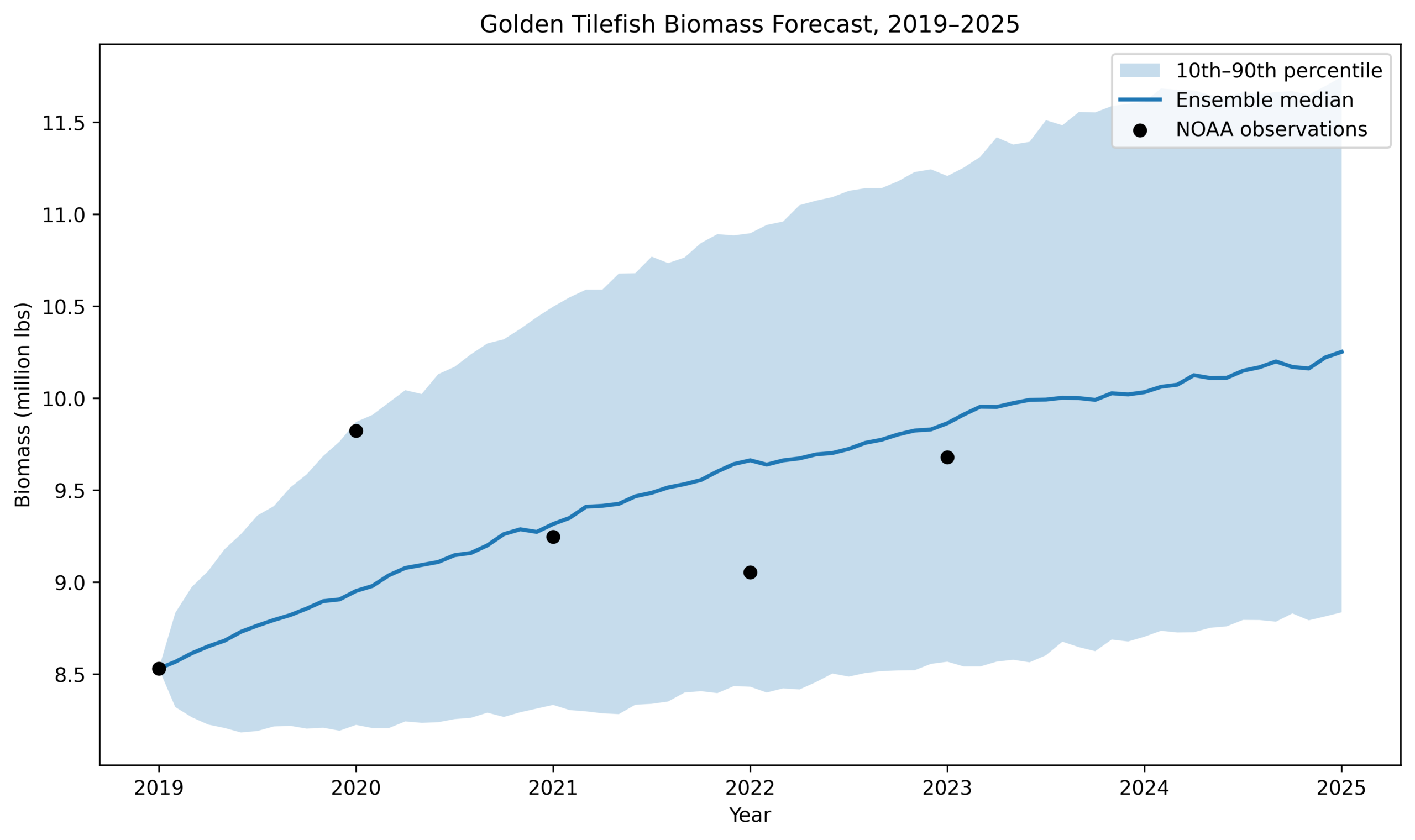
Figure 1 shows that the ensemble median remained within the general range of the observed Golden Tilefish biomass series while the prediction interval broadened over time as stochastic uncertainty accumulated. The final 1,000-member ensemble produced median biomass estimates of 8.95, 9.32, 9.66, and 9.86 million lbs for 2020–2023, respectively, compared with NOAA estimates of 9.82, 9.25, 9.05, and 9.68 million lbs. The corresponding signed percent errors were −8.86%, 0.75%, 6.74%, and 1.92%. All NOAA biomass estimates for the evaluation period fell within the corresponding 10th–90th percentile prediction intervals.

Across 2020–2023, the ensemble-median forecast produced a mean absolute error (MAE) of 433,676 lbs, a root mean squared error (RMSE) of 540,360 lbs, a mean bias of −1,297 lbs, and a maximum absolute annual error of 869,945 lbs. The standard deviations of MAE, RMSE, and bias were approximately 376,858 lbs, 411,985 lbs, and 727,605 lbs, respectively, across individual stochastic trajectories. These results demonstrate that individual stochastic realizations can vary substantially even when the ensemble median remains comparatively close to the observed biomass series. Forecast performance of the stochastic Gompertz model was also compared with deterministic Gompertz and naive persistence baselines, as shown in Figure 2.

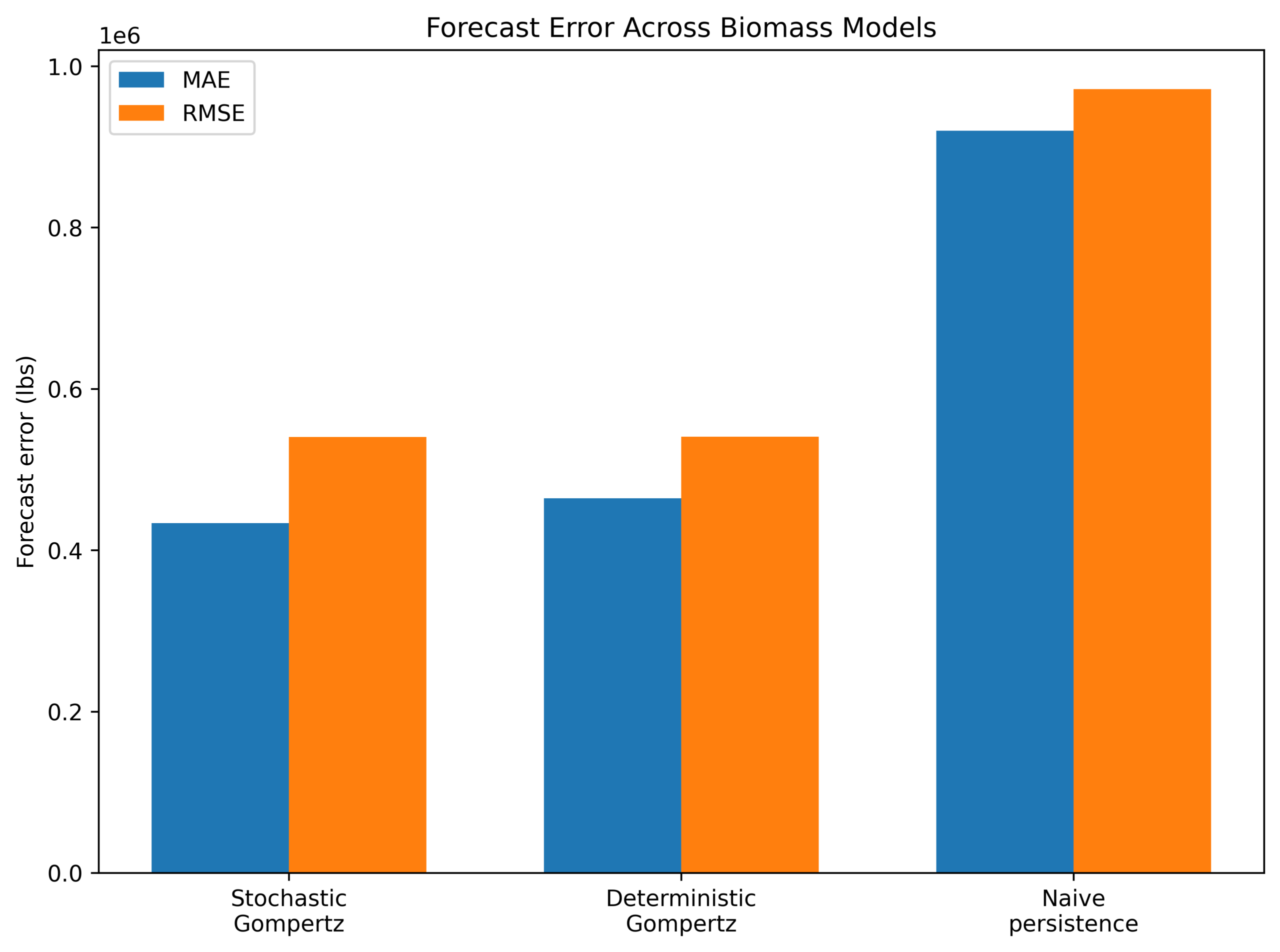
The corresponding forecast performance metrics for the stochastic model and both baseline models are summarized in Table 2.

Model	MAE (lbs)	RMSE (lbs)	Bias (lbs)	Mean absolute % error
Stochastic Gompertz	433,676	540,360	-1,297	4.57%
Deterministic Gompertz	464,275	540,623	51,693	4.90%
Naive Persistence	919,878	971,429	-919,878	9.64%

The stochastic Gompertz model produced lower overall forecast error than both baseline approaches. Across 2020–2023, the stochastic model achieved an MAE of 433,676 lbs and an RMSE of 540,360 lbs. This is compared with an MAE of 464,275 lbs and an RMSE of 540,623 lbs for the deterministic Gompertz baseline.  With an MAE of 919,878 lbs and an RMSE of 971,429 lbs, the naive persistence model performed substantially worse. The stochastic model also exhibited a mean bias of −1,297 lbs, compared with 51,693 lbs for the deterministic model and −919,878 lbs for the persistence baseline. Mean absolute percentage error was 4.57%, 4.90%, and 9.64% for the stochastic, deterministic, and persistence models, respectively. Incorporating stochastic environmental variability provided a modest improvement over the corresponding deterministic Gompertz formulation and a substantially larger improvement over the persistence benchmark.  The results of the one-at-a-time parameter sensitivity analysis are summarized in Table 3.

Parameter	Perturbation	MAE (lbs)	RMSE (lbs)	Bias (lbs)	MAPE (%)	Mean 10th-90th PI widths (lbs)
Baseline	—	433,676	540,360	-1,297	4.57	2,229,366
	−10%	492,781	622,509	−467,687	5.10	2,116,014
	+10%	775,919	816,438	443,435	8.25	2,337,652
	−10%	379,312	527,140	−97,673	3.98	2,274,415
	+10%	506,579	575,942	98,598	5.35	2,202,738
	−10%	440,529	541,712	8,946	4.64	2,008,015
	+10%	425,988	538,903	−12,628	4.48	2,450,189
Harvest Scaling	−10%	455,565	549,699	27,798	4.80	2,232,638
Harvest Scaling	+10%	411,442	532,470	−30,826	4.33	2,226,346

The one-at-a-time sensitivity analysis indicated that forecast performance was most responsive to changes in the asymptotic biomass parameter a. A 10% decrease in a increased RMSE from 540,360 to 622,509 lbs and a 10% increase raised RMSE to 816,438 lbs. Forecast error showed a smaller response to perturbations in b, with RMSE ranging from 527,140 to 575,942 lbs for -10% and +10% changes.  When examining the σ and the harvest-scaling coefficient, there were relatively small changes in point-forecast error. Environmental stochasticity had a clearer influence on forecast uncertainty: decreasing σ by 10% reduced the mean 10th–90th percentile interval width from 2.23 million to 2.01 million lbs.  Increasing σ by 10% widened it to 2.45 million lbs. The sensitivity analysis shows that point forecasts are particularly sensitive to the assumed asymptotic biomass level and that the primary influence of the stochasticity parameter is the width of the forecast distribution.

Discussion

The stochastic and deterministic Gompertz models produced similar point-forecast performance over the 2020–2023 evaluation period. Both performed substantially better than the naive persistence baseline. The stochastic model achieved an MAE of 433,676 lbs and an RMSE of 540,360 lbs compared with an MAE of 464,275 lbs and an RMSE of 540,623 lbs for the deterministic Gompertz baseline. The naive persistence baseline performed substantially worse, with an MAE of 919,878 lbs and an RMSE of 971,429 lbs. RMSE values were nearly identical between the stochastic and deterministic models and the stochastic model produced a small reduction in MAE. The stochastic model also exhibited a mean bias of −1,297 lbs compared with 51,693 lbs for the deterministic model. These results show that the main advantage of the stochastic Gompertz model is its ability to communicate forecast uncertainty through a distribution during predication intervals rather than an improvement in point-forecast accuracy.  

An important feature of the stochastic model is that it produces a distribution of possible biomass trajectories rather than only a single deterministic projection. In the final 1,000-member ensemble, all NOAA-reported biomass estimates from 2020 through 2023 fell within the corresponding 10th–90th percentile prediction intervals. The widening prediction intervals observed across the forecast horizon demonstrate the importance of representing uncertainty and the magnitude of the potential errors which may come from relying on a single narrow deterministic biomass trajectory. Accounting for uncertainty is particularly important for fish populations which are subject to environmental variability and episodic ecological shocks²³. Across the individual stochastic trajectories, the relatively large standard deviations in MAE, RMSE, and bias demonstrate that individual outcomes can differ substantially from the median.  This is the case even though the median forecast remained relatively close to the observed biomass series.  That is to say, even if the median forecast appears accurate, it may not be precise, and predicted results may fall along a wide distribution. For fisheries management, these distributions may be more informative than point forecasts alone because they explicitly represent uncertainty in future biomass states.

The DGM component serves a complementary role to the Monte Carlo biomass forecasts. Whereas Monte Carlo simulation generates the forecast distribution of future biomass states, DGM approximates the value function associated with the management threshold. The value function is the expected penalty associated with biomass falling below the specified management threshold.  It provides a means of interpreting stochastic biomass dynamics in terms of management risk. This difference is important because the biomass trajectories presented in the Results were not generated by the neural network itself. Instead, the stochastic Gompertz model provides the forecasting engine, while DGM provides a mesh-free numerical approach for approximating the associated threshold-risk value function¹³.

This study has several limitations. First, the environmental stochasticity parameter (σ) and mean-reversion parameter (b) are assumed constant over the simulation period.  The future harvest pressure is also represented through fixed year-specific landings and a calibrated harvest-scaling factor. These assumptions may not capture longer-term climatic shifts, changes in recruitment, altered fishing behavior, or future management actions. In addition, model calibration and evaluation were based on a relatively short series of annual biomass observations, which limits the extent to which out-of-sample predictive performance can be established.

Also, climate-driven changes in stock distribution may also alter spawning biomass, catch variability, and the performance of harvest-control rules²⁴. Unaccounted for time-varying parameters and environmental covariates such as sea-surface temperature, recruitment indices, or habitat conditions may be particularly important because climate and ecosystem changes can contribute to uncertainty in fisheries stock assessments²⁵. Recent evaluations of fisheries management procedures have shown the importance of developing strategies that remain robust when climate change violates assumptions of stationarity²⁶. Finally, the present formulation also considers a single-species biomass process. Extension to multispecies interactions could provide a basis for broader ecosystem-based management applications.

The stochastic Gompertz model predicts Golden Tilefish biomass while incorporating uncertainty in future biomass projections. In addition, the 1,000-member Monte Carlo ensemble provided prediction intervals that captured all NOAA-reported biomass estimates during the evaluation period, illustrating the additional value in information provided by probabilistic forecasts beyond a single trajectory. DGM provides a method for approximating a management value function which is associated with biomass-threshold risk rather than serving as the direct biomass forecasting engine. Stochastic biomass forecasts and threshold-based risk measures can the combined to support uncertainty-aware fisheries analysis. Validation using longer time series, broader parameter-uncertainty analyses, and additional fisheries datasets will be necessary to determine the broader utility of the approach.

References

1. T. J. Quinn. Ruminations on the development and future of population dynamics models in fisheries. Natural Resource Modeling. Vol. 16, pg. 341–392, 2003, https://doi.org/10.1111/j.1939-7445.2003.tb00119.x. [↩]
2. K. M. Privitera-Johnson, A. E. Punt. Leveraging scientific uncertainty in fisheries management for estimating among-assessment variation in overfishing limits. ICES Journal of Marine Science. Vol. 77, pg. 515–526, 2020. https://doi.org/10.1093/icesjms/fsz237. [↩]
3. A. Kokkalis, A. Eikeset, A. Thygesen, O. R. Eigaard, M. Andersen, J. R. Nielsen. Time-variant productivity in biomass dynamic models on seasonal and long-term scales. ICES Journal of Marine Science. Vol. 77, pg. 174–187, 2020. https://doi.org/10.1093/icesjms/fsz154. [↩]
4. K. K. Holsman, A. C. Haynie, A. B. Hollowed, J. C. P. Reum, K. Aydin, A. J. Hermann, W. Cheng, A. Faig, J. N. Ianelli, K. A. Kearney, A. E. Punt. Ecosystem-based fisheries management forestalls climate-driven collapse. Nature Communications. Vol. 11, 4579, 2020. https://doi.org/10.1038/s41467-020-18300-3. [↩]
5. J. S. Link, M. A. Karp, P. Lynch, W. E. Morrison, J. Peterson. Proposed business rules to incorporate climate-induced changes in fisheries management. ICES Journal of Marine Science. Vol. 78, pg. 3562–3580, 2021. https://doi.org/10.1093/icesjms/fsab219. [↩]
6. M. Sun, Y. Li, Y. Ren, Y. Chen. Rebuilding depleted fisheries towards BMSY under uncertainty: harvest control rules outperform combined management measures. ICES Journal of Marine Science. Vol. 78, pg. 2218–2232, 2021. https://doi.org/10.1093/icesjms/fsaa078. [↩]
7. S. Carpenter, W. Brock, P. Hanson. Ecological and social dynamics in simple models of ecosystem management. Conservation Ecology. Vol. 3, pg. 31, 1999, https://www.jstor.org/stable/26271717. [↩]
8. V. Riquelme, T. J. Quinn, H. Ramirez C. The role of uncertainty in the design of sustainable and precautionary management strategies for fisheries. Natural Resource Modeling. Vol. 33, e12279, 2020, https://doi.org/10.1111/nrm.12279. [↩]
9. M. D. Gunzburger, C. G. Webster, G. Zhang. Stochastic finite element methods for partial differential equations with random input data. Acta Numerica. Vol. 23, pg. 521–650, 2014, https://doi.org/10.1017/S0962492914000075. [↩]
10. J. Han, A. Jentzen, E. W. Solving high-dimensional partial differential equations using deep learning. Proceedings of the National Academy of Sciences. Vol. 115, pg. 8505–8510, 2018, https://doi.org/10.1073/pnas.1718942115. [↩]
11. D. Zhang, L. Guo, G. E. Karniadakis. Learning in modal space: Solving time-dependent stochastic PDEs using physics-informed neural networks. SIAM Journal on Scientific Computing. Vol. 42, pg. A639–A665, 2020. https://doi.org/10.1137/19M1260141. [↩]
12. L. Lu, X. Meng, Z. Mao, G. E. Karniadakis. DeepXDE: A deep learning library for solving differential equations. SIAM Review. Vol. 63, pg. 208–228, 2021. https://doi.org/10.1137/19M1274067. [↩]
13. J. Sirignano, K. Spiliopoulos. DGM: A deep learning algorithm for solving partial differential equations. arXiv. 2018, https://doi.org/10.48550/arXiv.1708.07469. [↩] [↩] [↩]
14. M. R. Payne, G. Danabasoglu, N. Keenlyside, D. Matei, A. K. Miesner, S. Yang, et al. Skilful decadal-scale prediction of fish habitat and distribution shifts. Nature Communications. Vol. 13, 2660, 2022. https://doi.org/10.1038/s41467-022-30280-0. [↩]
15. S. Brodie, M. Pozo Buil, H. Welch, S. J. Bograd, E. L. Hazen, J. A. Santora, R. Seary, I. D. Schroeder, M. G. Jacox. Ecological forecasts for marine resource management during climate extremes. Nature Communications. Vol. 14, 7701, 2023. https://doi.org/10.1038/s41467-023-43188-0. [↩]
16. K. M. C. Tjørve, E. Tjørve. The use of Gompertz models in growth analyses, and new Gompertz-model approach: An addition to the Unified-Richards family. PLOS ONE. Vol. 12, e0178691, 2017, https://doi.org/10.1371/journal.pone.0178691. [↩]
17. A. Al-Aradi, A. Correia, D. Naiff, G. Jardim, Y. Saporito. Solving nonlinear and high-dimensional partial differential equations via deep learning. arXiv. 2018, https://doi.org/10.48550/arXiv.1811.08782. [↩]
18. M. H. Holden, J. M. Conrad. Optimal escapement in stage-structured fisheries with environmental stochasticity. Mathematical Biosciences. Vol. 269, pg. 76–85, 2015, https://doi.org/10.1016/j.mbs.2015.08.021. [↩]
19. Z. Gao, L. Yan, T. Zhou. Failure-informed adaptive sampling for PINNs. SIAM Journal on Scientific Computing. Vol. 45, pg. A1971–A1994, 2023. https://doi.org/10.1137/22M1527763. [↩]
20. S. Wang, Y. Teng, P. Perdikaris. Understanding and mitigating gradient flow pathologies in physics-informed neural networks. SIAM Journal on Scientific Computing. Vol. 43, pg. A3055–A3081, 2021. https://doi.org/10.1137/20M1318043. [↩]
21. N. D. Ducharme-Barth, M. T. Vincent. Focusing on the front end: A framework for incorporating uncertainty in biological parameters in model ensembles of integrated stock assessments. Fisheries Research. Vol. 255, 106452, 2022. https://doi.org/10.1016/j.fishres.2022.106452. [↩]
22. NOAA. Stock SMART. NOAA Fisheries. 2025. Accessed December 22, 2025. https://apps-st.fisheries.noaa.gov/stocksmart/?stockname=Tilefish%20-%20Mid-Atlantic%20Coast&stockid=10385. [↩]
23. B. Dennis. Allee effects: Population growth, critical density, and the chance of extinction. Natural Resource Modeling. Vol. 3, pg. 481–538, 1989, https://doi.org/10.1111/j.1939-7445.1989.tb00119.x. [↩]
24. N. S. Jacobsen, K. N. Marshall, A. M. Berger, C. Grandin, I. G. Taylor. Climate-mediated stock redistribution causes increased risk and challenges for fisheries management. ICES Journal of Marine Science. Vol. 79, pg. 1120–1132, 2022. https://doi.org/10.1093/icesjms/fsac029. [↩]
25. L. Kerr, M. Barajas, J. Wiedenmann. Coherence and potential drivers of stock assessment uncertainty in Northeast US groundfish stocks. ICES Journal of Marine Science. Vol. 79, pg. 2217–2230, 2022. https://doi.org/10.1093/icesjms/fsac140. [↩]
26. C. D. Peterson, N. Klibansky, M. T. Vincent, J. F. Walter III. Climate-readiness of fishery management procedures with application to the southeast US Atlantic. ICES Journal of Marine Science. Vol. 82, Issue 1, fsae154, 2025. https://doi.org/10.1093/icesjms/fsae154. [↩]