Multi-dimensional Scientific Data Compression using Lorenzo Predictor and RLE

Abstract

As processors have become increasingly powerful compared to storage systems, being able to access data efficiently for scientific applications has become more important than ever. Data reduction techniques address this issue by minimizing the amount of data that must be stored by simulation and subsequently retrieved by scientific data analytics, thereby reducing the time to knowledge. Many existing lossy compressors use linear interpolation to predict the value of a data point and then compress the difference between the predicted and actual values using an entropy encoder, like Huffman tree. This 1D predictor serves as the baseline in this work, since it is a common building block used in many lossy compressors, including SZ, and represents the common approach. Given that linear interpolation does not fully take advantage of the locality in the data, there were previous works that explored the Lorenzo predictor. However, it is unclear how Lorenzo will perform when used with run-length encoding, which is a commonly used entropy encoder. Although there were prior works on hybrid predictive and encoding schemes, such as SZ, the unique combination of Lorenzo and run-length encoding has not been attempted. This paper develops a 2D Lorenzo predictor, which uses neighboring values in the 2D space for prediction, and run-length encoding for scientific data compression. Based on the Lorenzo prediction, the error is quantized into an integer bucket based on a prescribed error tolerance. The quantized values are subsequently compressed using run-length encoding to remove the redundancy in data. We evaluate four real scientific datasets, CESM-ATM, NYX, QMCPACK, and HURRICANE, and the Lorenzo prediction and run-length encoding results in a substantial improvement in compression ratio, e.g., by 4.7X for the NYX data, as compared to the 1D compression, using the relative error bound, defined as the proportion of the absolute error and the maximum absolute of all data points.

Keywords: High-performance computing, data reduction, scientific data analytics

Introduction

The rapid advancement of various types of scientific instruments, particularly the new exascale high-performance computing (HPC) systems, has led to an exponential increase in the volume of data generated across various disciplines, such as climate simulation and molecular dynamics^1,2. Computing capabilities have improved with accelerators such as GPUs and TPUs, but data storage and I/O systems have not scaled at the same rate^3,4. As a result, managing data efficiently, particularly with storage, retrieval, and transfer, has become a critical factor that limits scientific productivity.

To address these challenges, data reduction techniques have been redesigned in the past decade, primarily to deal with the I/O bottleneck on exascale systems^3,5. These techniques share a common theme: to lower data overhead without significantly compromising the outcomes of data analysis. Among these techniques, floating-point lossy compression has gained widespread attention due to its ability to reach substantially higher compression ratios as compared to lossless methods^5,4.

This paper presents an empirical study of lossy compression for two-dimensional floating-point data based on the Lorenzo predictor and run-length encoding (RLE). Many existing lossy compressors use linear or Lorenzo prediction followed by Huffman encoding, but their relative performance when paired with RLE, a common entropy encoder, remains unclear^6,7,8. Another widely used compressor, FPZIP⁴, takes a different approach, predicting each value from previously seen neighbors using higher-order Lagrange extrapolation and encoding the residual directly as a floating-point number rather than quantizing it into buckets. To this end, this paper implements a 2D Lorenzo predictor, which uses neighboring values in the 2D space for prediction, and adopts RLE for lossless compression written in C/C++. In particular, after the Lorenzo prediction, the error is quantized into an integer bucket based on a prescribed error tolerance. The quantized values are subsequently compressed by identifying runs and replacing them by run-length pairs to reduce the storage footprint. The core contributions of this work are as follows: 1) This paper conducts an empirical performance study of a unique combination of lossy compression methods: Lorenzo predictor and RLE. 2) This work evaluates four real datasets from different disciplines and shows that Lorenzo is highly beneficial when RLE is used for entropy encoding, as compared to the simple 1D linear predictor.

Methods

In this section, we describe the algorithms for 1D predictor, Lorenzo predictor, RLE as well the decompression process.

1D predictor

Algorithm 1 illustrates the pseudocode for the 1D predictor, which serves as the baseline for performance comparison in this work. Overall, the idea is to compress data by predicting the data value based on the previous two data points. This algorithm takes the input data d, the number of data points n, and absolute error tolerance e, as inputs, and produces the quantized data delta.  Line 1 initializes an array for the delta, and Line 2 allocates two variables nm1 and nm2, which keep track of the values of two previous data points, respectively. From Lines 3 to 12, the code loops through all the data points and performs the 1D predictive encoding. In particular, Line 4 retrieves the value of data point i from the input data, followed by a linear prediction (2*nm1 – nm2) at Line 5. The delta is calculated by subtracting the current value from the predicted value.  Then, at Line 6, the delta is checked to determine whether it is positive or negative. Line 7 quantizes the error into a bucket through a number of steps. First, the function fabs(diff) returns the absolute value of the delta and adds e, resulting in the offset of delta with regard to bucket 0. Then it divides this by the size of a bucket 2e to calculate the bucket ID. This step keeps the error within a controlled bound. Across this paper, we use implicit type conversion to truncate a float to an integer.In Line 8, we reconstruct the data point to the original value by adding the quantized error, which is represented by bucket * 2e, to the delta. This reconstructed value will be used for the prediction of the next data point to ensure the error is not propagated and amplified for the subsequent data points. Then the bucket is stored in the delta array, in Line 9.Following this, the algorithm updates its memory by shifting nm1 and nm2 and setting nm1 to the reconstructed value, in Lines 10 and 11. After processing all data points, the algorithm returns delta, which now holds the quantized delta.

Algorithm 1: 1D Predictor
Input: input data d, total number of data points n, error tolerance e
Output: quantized delta
1.	delta = {}
2.	float nm1= 0.0, nm2 = 0.0
3.	for i = 0 to n - 1: 
4.	current = d[i]
5.	     d = current - (2 * nm1 - nm2)
6.	     if d >= 0 then sign = 1 else sign = -1
7.	     bucket = sign * (fabs (d) + e) / (2 * e)
8.	     reconstructed = (2 * nm1 - nm2) + bucket * 2 * e
9.	     delta [i] = bucket
10.	     nm2 = nm1
11.	     nm1 = reconstructed
12.	end for
13.	return delta

To walk through how prediction, quantization, reconstruction, and the state update fit together, here is a small example with an absolute error bound e = 0.5 and three input data points: d[0] = 10.0, d[1] = 8.2, d[2] = 12.5. The first two points do not have any prior history to predict from, so they get stored directly and reconstructed the same way, which sets nm2 = d[0] = 10.0 and nm1 = d[1] = 8.2. For the third point, d[2] = 12.5, pred = 2*nm1 − nm2 = 2(8.2) − 10.0 = 6.4. The residual is diff = d[2] − pred = 12.5 − 6.4 = 6.1. Quantizing gives bucket = (int)((|diff| + e) / (2e)) = (int)((6.1 + 0.5) / 1.0) = (int)(6.6) = 6. The cast to int truncates toward zero, which works as a floor here since the value inside is always non-negative. Reconstruction gives reconstructed = bucket × 2e = 6 × 1.0 = 6.0. Since the residual was positive, the reconstructed value is pred + reconstructed = 6.4 + 6.0 = 12.4. The reconstruction error is |12.4 − 12.5| = 0.1, which stays within the bound. Finally, the state updates for the next point: nm2 becomes the old nm1 (8.2), and nm1 becomes 12.4, so future predictions use decompressed values instead of the originals.

Algorithm 2: Lorenzo 2D Predictor
Input: input data d, size of Y dimension y_dim, size of X dimension x_dim, error tolerance e
Output: quantized delta
1.	data_temp = d
2.	delta = {}
3.	for i = 0 to y_dmi - 1:
4.	     for j = 0 to x_dim – 1:
5.	          if i – 1 >= 0 then im1j = data_temp[i - 1][j] else im1j = 0.0
6.	          if j - 1 >= 0 then ijm1 = data_temp[i][j - 1] else ijm1 = 0.0
7.	          if i – 1 >= 0 and j – 1 >= 0 then
8.	               im1jm1 = data_temp[i - 1][j - 1]
9.	          else
10.	               im1jm1 = 0.0
11.	          predicted = im1j + ijm1 – im1jm1
12.	          current = data_temp[i][j]
13.	          resid = current - predicted
14.	          if resid >= 0 then sign = 1 else sign = -1
15.	          bucket = truncate(sign * (fabs(resid) + e) / (2 * e))

16.	          reconstructed = predicted + bucket * 2 * e
17.	          delta[i][j] = bucket
18.	          data_temp[i][j] = reconstructed
19.	     end for
20.	end for

21.	return delta 

Lorenzo predictor

Algorithm 2 illustrates the pseudocode for the Lorenzo 2D predictor. This algorithm reduces the storage size of the data by converting the data into integer buckets of prediction error, while keeping the reconstruction error within a chosen tolerance e. It takes the input data d, the size of the X and Y dimensions, x_dim and y_dim, respectively, as well as the absolute error tolerance e as input. In turn, it produces the quantized data delta.

Line 1 copies the data d to data_temp, so we can modify the data without losing the original dataset. Line 2 creates an output array delta to store the buckets. Lines 3-20 are a loop that analyzes each data point in the 2D space and processes it using the Lorenzo prediction. Specifically, Lines 3 and 4 create a nested loop that iterates through all the data points in the 2D space. In Lines 5-10, the code retrieves the values of adjacent data points, and if an adjacent data point does not exist, we set it to zero. In particular, Line 5 gets the value above the current point, Line 6 gets the value to the left of the data point, and Line 7 gets the top-left diagonal value. Using all this information, Line 11 uses the formula of the Lorenzo predictor to make the prediction. Then, Line 12 retrieves the actual value of the current data point.  Line 13 computes the prediction error, which is the difference between the real and predicted data, and stores it in the variable resid. Line 14 then checks whether the error is a positive or negative value. Line 15 converts the error into a quantized bucket, similar to what Algorithm 1 does. To ensure consistent results when running the algorithm, Line 16 creates an approximate value using the bucket created by Line 15. Lines 17 and 18 store the final compressed value as the output and then replace the original value with the newly reconstructed one.

Formally, the Lorenzo predictor at row i and column j is given by

predicted = D[i][j-1] + D[i-1][j] − D[i-1][j-1]

using the left, top, and top-left diagonal neighbors, taken from already-decompressed values so error does not propagate. The residual is resid = D[i][j] − predicted, quantized into a bucket as before.

At a boundary data point (i = 0 or j = 0), its missing neighbors are set to zero (but the boundary itself is not). We chose zero padding for its simplicity, since it only needs a bound check. Replication padding (using the nearest valid neighbor) and extrapolation would likely predict better at boundaries. However, for a large dataset, the number of boundary data points is relatively low, and they are not expected to result in substantially higher performance, albeit at a higher cost for extrapolation at the boundary.

The Lorenzo predictor works well in smooth regions, where residuals stay small and repetitive, helping RLE. In regions with sharp gradients or discontinuities, the assumption breaks down, producing larger, less repetitive residuals and shorter RLE runs. A second-order predictor can reduce this error with an added cost. This is left for future study.

Algorithm 3: Run Length Encoding (RLE)
Input: 2D integer array quantized_2d, number of rows y_dim, number of columns x_dim, output_size 
Output: 1D run-length encoded array rle_output 
1.	num_elements = y_dim * x_dim
2.	quantized = new array of size num_elements
3.	if quantized == null then 
4.	print “Malloc error”
5.	exit program
6.	end if 
7.	for i = 0 to y_dim -1:
8.	for j =.0 to x_dim – 1:
9.	quantized[i * x_dim + j] = quantized_2d[i][j]
10.	end for
11.	end for
12.	rle_output = new array of size 2 * num_elements
13.	i = 0
14.	j = 0 
15.	while I < num_elements:
16.	len = 1
17.	bucket_id = quantized[i} 
18.	while i != num_elements – 1 and quantized[i+1] == bucket_id:
19.	i = i +1
20.	len = len + 1 
21.	end while
22.	rle_output[j] = bucket_id 
23.	rle_output[j+1] = len
24.	j = j + 2
25.	i = i + 1 
26.	end while
27.	output_size = l
28.	return rle_output

RLE

Algorithm 3 describes the steps to perform run-length encoding for quantized data. The input of the algorithm is quantized data quantized_2d, sizes of Y and X dimensions, y_dim and x_dim, respectively. The output is the RLE encoded data rle_output. Line 1 calculates the total number of elements in the data and Line 2 allocates an array for storing the linearized quantized data. From Lines 3 to 16, we apply the RLE encoding. Line 7 identifies the current bucket ID, and Lines 8 to 11 advance the index i through all consecutive elements with the same bucket_id. Once the run ends, the run length is stored, and the pair (bucket_id, len) is stored in rle_output (Lines 12 and 13). The outer loop then continues from the updated i, which already points to the next unprocessed element.

Decompression

The decompression process is the reverse process of compression. Namely, we conduct run-length decoding first, followed by predictive decoding. In particular, we use linear or Lorenzo prediction, respectively, for reconstruction. After that the decompressed data will be copied to the user space.

Results

Error bound	Raw input size	Compressed byte size	# of RLE pairs	Compress ratio	Compress time	Decompress time
0.1	25920000	414688	414688	62.5	0.24	0.085
0.01	25920000	2997784	2997784	8.6	0.24	0.086
0.001	25920000	17526408	17526408	1.5	0.25	0.093
0.0001	25920000	28503408	28503408	0.9	0.27	0.0999

Error bound	Raw input size	Compressed byte size	# of RLE pairs	Compress ratio	Compress time	Decompress time
0.1	536870912	72688	72688	7385.96	4.42	1.70
0.01	536870912	944272	944272	568.56	4.5	1.82
0.001	536870912	17305056	17305056	31.02	4.77	1.86
0.0001	536870912	167556672	167556672	3.20	4.73	1.99

Error bound	Raw input size	Compressed byte size	# of RLE pairs	Compress ratio	Compress time	Decompress time
0.1	630737280	38014424	38014424	16.59	5.55	2.26
0.01	630737280	273647696	273647696	2.30	5.67	2.46
0.001	630737280	560476184	560476184	1.13	5.92	2.75
0.0001	630737280	742450968	742450968	0.85	6.14	2.83

Error bound	Raw input size	Compressed byte size	# of RLE pairs	Compress ratio	Compress time	Decompress time
0.1	100000000	2853192	2853192	35.05	0.78	0.33
0.01	100000000	10646624	10646624	9.39	0.83	0.33
0.001	100000000	19301376	19301376	5.18	0.87	0.33
0.0001	100000000	25576864	25576864	3.91	0.85	0.34

Dimensions	Compression ratio	Compression throughput (MB/s)
2285280×69	16.59	106.34
1142640×138	12.72	105.37
571320×276	11.238216	104.207401
285660×552	10.185582	105.667016
142830×1104	9.354004	106.722206

Error bound	Max absolute error	Max pointwise relative error	RMSE	PSNR
0.1	0.1000	0.1750	0.0573	19.98
0.01	0.0100	0.0175	0.0055	40.29
0.001	0.0010	0.0018	0.0005	60.50
0.0001	0.0001	0.0002	0.0001	80.47

Error bound	Max absolute error	Max pointwise relative error	RMSE	PSNR
0.1	0.1000	0.000001	0.0572	126.13
0.01	0.0112	0.000000	0.0058	146.05
0.001	0.0039	0.000000	0.0006	166.05
0.0001	0.0024	0.000000	0.0001	186.05

Error bound	Max abs error	Max pointwise relative error	RMSE	PSNR
0.1	0.1000	0.0066	0.0305	59.98
0.01	0.0100	0.0007	0.0044	76.82
0.001	0.0010	0.0001	0.0005	95.13
0.0001	0.0001	0.00001	0.0001	114.46

Error bound	Max abs error	Max pointwise relative error	RMSE	PSNR
0.1	0.0020	1.0000	0.0001	31.69
0.01	0.0020	1.0000	0.0001	31.69
0.001	0.0010	0.4883	0.0001	31.85
0.0001	0.0001	0.0488	0.0000	43.55

Discussion

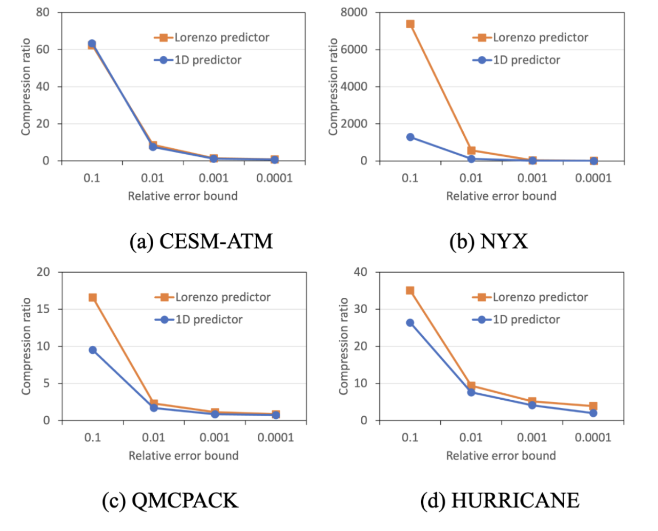
Figure 1 shows the compression ratios of the four scientific datasets using both Lorenzo (in orange) and 1D predictors (in blue). We vary the pointwise relative error bound from 0.1 to 0.0001 to test a wide range of error tolerance and understand how it will impact the compression performance. In particular, the relative error bound is the proportion of the absolute error and the maximum absolute of all data points. Overall, the Lorenzo predictor yields significantly higher compression ratios than the 1D predictor, particularly when the error tolerance is high. For example, for NYX, as shown in Figure 1(b), at a relative error of 0.1, the compression ratio of the Lorenzo predictor is 5X higher than that of the 1D predictor. As the error bound tightens, the gain of Lorenzo becomes smaller, suggesting that for small error tolerance, the prediction will unlikely result in repeated quantization buckets, thus resulting in diminishing gain of Lorenzo. On the other hand, as the relative error bound reduces, the overall trend is that the compression ratio also reduces. This is because as the error bound becomes tighter, the size of each quantization bucket becomes smaller, resulting in data points being more likely to be represented by different buckets. Therefore, the length of a run becomes likely shorter, and the backend RLE becomes less effective in reducing the footprint of data.

The improvement of the Lorenzo predictor over the 1D predictor can be understood as follows. The 2D Lorenzo predictor exploits spatial locality in both dimensions simultaneously, producing more accurate predictions for smoothly varying data–the type most commonly produced by scientific simulations. When prediction accuracy is higher, the prediction errors are smaller in magnitude and more likely to cluster in a narrow range of quantization buckets. Consecutive data points that fall into the same bucket form a run in RLE, and longer runs translate directly to higher compression ratios. The 1D predictor, by contrast, considers data only along a single axis and misses correlations in the orthogonal direction, yielding less accurate predictions and less repetitive quantized sequences. The diminishing advantage of Lorenzo at tight error bounds is also analytically interpretable. As the relative error bound tightens, the quantization bucket width 2e decreases proportionally. With a finer quantization grid, even small differences between adjacent data values assign those values to different buckets, shortening RLE runs regardless of predictor accuracy. At the tightest bound evaluated (0.0001), both predictors produce comparably non-repetitive quantized sequences.

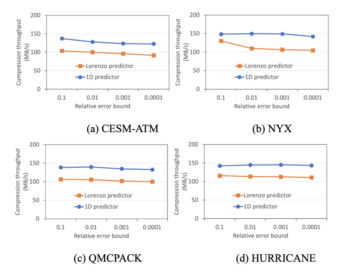
Figure 2 shows the compression throughput of both predictors. As expected, the Lorenzo predictor results in lower throughput compared to the 1D Predictor.  The reason is that the Lorenzo predictor involves more data points in prediction and therefore has higher computation overhead, as compared to 1D predictor. Additionally, there is serialization overhead involved when converting 2D to 1D for entropy encoding. On the other hand, the compression throughput is not sensitive to the error bound, since the algorithm complexity remains identical across different error bounds.

We note that our implementation is not intended as a direct competitor to production-quality compressors such as SZ⁹ or ZFP¹⁰. SZ employs the Lorenzo predictor with Huffman encoding, which typically achieves substantially higher compression ratios than our RLE-based implementation at equivalent error bounds; Huffman encoding adapts to the full distribution of bucket IDs rather than exploiting only consecutive runs. ZFP uses a different approach that is distinct from prediction-quantization principles. A quantized comparison with SZ and ZFP is identified as future work.

From Tables 1 to 4, we vary the pointwise relative error bound from 0.1 to 0.0001 to test a wide range of error tolerance and understand how it will impact the compression performance for each dataset. The performance metrics we collected include raw input size, compressed byte size, number of RLE pairs, compression ratio, compression time, and decompression time.

Table 5 shows the impact of different reshaping of data on the compression performance for QMCPACK, where we vary the size of dimensions of the data. As we expected, the reshaping can impact some of the compression ratios. However, since multi-dimensional compression is not the focus of this paper, we leave it for future engineering effort to improve our work.

From Tables 6 to 9, we list maximum absolute error, maximum pointwise relative error, RMSE, PSNR for reconstructed data and verify that the pointwise relative error that we enforce in this work is satisfied. Other types of error are listed here for possible future comparisons.

Literature Review

Data reduction over the past few years has attracted considerable interest from the HPC community. SZ⁹ uses multiple prediction algorithms with Huffman encoding¹¹, and was later split into a modular framework, SZ2, so the predictor and encoder can be swapped independently¹². ZFP¹⁰ instead transforms small blocks of data and encodes directly, building on earlier work exploiting the bit structure of floating-point arrays⁴. MGARD¹³ and TTHRESH¹⁴ use multigrid or tensor decomposition rather than a pointwise predictor, and cuSZ¹⁵ and cuZSp¹⁶ are GPU versions of this pipeline. We are not aiming to compete with mature compressors like SZ and ZFP here, just isolate how one specific predictor-encoder pairing performs.

The predictor used in this paper builds on the Lorenzo predictor, first proposed by Ibarria et al. for compressing large n-dimensional scalar fields². SZ adopted this predictor in later versions and turned it further to get better compression ratios⁵. A simple 1D predictor only looks at the previous one or two data points along a single axis, while the Lorenzo predictor uses neighboring values from multiple directions, which captures the local smoothness common in simulation data better. This is the same comparison we test in the paper, a 1D predictor against a 2D Lorenzo predictor, under the same error bounds.

Most existing lossy compressors pair the predictor with Huffman coding¹¹ or arithmetic coding¹⁷, since both handle the biased distribution of quantized prediction errors well. Run-length encoding hasn’t gotten as much attention as a backend for scientific data, even though it can work well when quantized values form long runs, which is what we see happen at looser error bounds in our results. A couple of recent papers have looked at improving RLE through selective encoding⁶ or preprocessing steps that make runs longer⁷, building on older work on RLE for structured data⁸.

A recent survey by Di et al.¹⁸ gives a broad overview of error-bound lossy compression, organizing over 40 compressors into organized categories of prediction. It confirms that prediction-based and transform-based methods have both been studied a lot, but the specific combination we study here, Lorenzo prediction with RLE instead of Huffman or arithmetic encoding, hasn’t been looked at.

The GPU side of this space has moved quickly in the last few years. cuSZ-i¹⁹ replaced the Lorenzo-style predictor with a multi-level interpolation scheme built specifically for GPU throughput, pushing far past what a CPU-side Lorenzo implementation like ours can do on speed. That comparison is not directly relevant here, since our implementation is single-threaded and runs on a CPU and we are not attempting to compete on throughput. However, it does show the research direction has shifted toward maximizing accelerator throughput rather than compression ratio on a single core.

A related idea is to tune the compressor around a specific downstream quality metric instead of a single fixed error bound, since not every scientific analysis is affected by error the same way. Liu et al. built a compression scheme that adjusts itself based on the target quality metric²⁰, rather than the raw error bound alone. We do not explore this here, since we deliberately keep the predictor and the error metric fixed to isolate the effect of RLE, but it points toward a natural next step for this line of work.

A separate and increasingly common research direction replaces the hand-designed predictor with a learned one. GWLZ²¹ trains a small neural network across a group of similar simulation output files and uses it to predict values that get quantized and encoded, which is essentially the same pipeline used in this paper with a learned model replacing Lorenzo. Huang et al. kept the classical prediction-and-quantization pipeline but swapped in a wavelet transform²², and reported the largest gains on data with sharp local variation, exactly where the Lorenzo predictor’s smoothness assumption breaks down. That last point matches what we observe in the Discussion: if the data is not locally smooth, prediction error grows, which results in low compression ratios.

On the entropy-encoding side, work on RLE itself has continued since the two papers discussed above. Poriev compared several ways of packing the run-length field and found that the best choice depends heavily on how repetitive the input already is²³, which is consistent with what we see across our four datasets: the number of RLE pairs grows quickly once the quantization bucket gets small enough that neighboring points stop landing in the same bucket.

A few other recent papers help explain why the specific datasets tested here behave the way they do. Applying lossy compression directly to cosmological simulation output in the same spirit as the NYX dataset used here, Pulido et al. found that compression ratio depends heavily on which physical field is being compressed rather than the error bound alone²⁴, which matches how much CESM-ATM, NYX, QMCPACK, and HURRICANE differ from each other in our own results even at the same error bound. A similar pattern shows up on the molecular dynamics data–a dedicated trajectory compressor built by Kokot et al. beats general-purpose compressors by exploiting the smooth, correlated motion of atoms from one frame to the next²⁵.

Two more papers focus on when to compress rather than how. Underwood et al. built a statistical model that predicts how compressible a dataset will be before actually running the compressor²⁶. This could help decide in advance whether the extra cost of Lorenzo prediction is worth it for a given dataset. Separately, a survey of how several application teams actually use lossy compression in practice found that acceptable error bounds vary a great deal by field and by what the data gets used for afterward²⁷, which is part of why we test error bounds spanning three orders of magnitude instead of a single fixed value.

Two more papers reinforce the predictor lineage behind this work. Tao et al. were among the first to combine a multidimensional predictor, of which Lorenzo is a special case, with error-controlled quantization in a single pipeline, and found that multidimensional prediction beats a 1D predictor on smooth scientific data with Huffman-based backend²⁸. Zhang et al. surveyed the broader HPC storage stack that lossy compression exists to relieve pressure on, and their finding that storage bandwidth keeps lagging behind compute growth on current systems is the same motivating problem raised in the Introduction²⁹.

Experimental Setup

Our experiments were conducted on an Apple MacBook Air with an Apple M3 processor and 16 GB of memory. This small platform was selected for the ease of code development and the lack of larger resources; the reported compression throughput figures therefore reflect single-core performance on a consumer laptop and should not be interpreted as large-scale results. Evaluating the algorithms on multi-core CPU nodes or GPU clusters, and profiling memory for very large datasets, are identified as directions for future work.

We tested our algorithms using real scientific data in single precision from Scientific Data Reduction Benchmarks (https://sdrbench.github.io/) and the description of data is as follows:

1) CESM-ATM: This dataset is produced by the Community Earth System Model (CESM), a widely used climate simulation framework. The dataset contains atmospheric variables generated through the simulation. In particular, we used a field called AEROD_v_1_1800_3600.dat for testing the performance of compression. This field is a 2D data with dimensions 1800×3600.

2) NYX: This dataset is produced by the NYX cosmological simulation, which is used to model the large-scale structure of the universe. In this study, baryon_density.f32 was used for testing. The data represents the distribution of baryonic matter in a simulated universe. The data is organized as a structured grid with dimensions 2,285,280 x 69. 

3) QMCPACK: This dataset is from the Quantum Monte Carlo software which is used for simulating the electronic structure of atoms, molecules, and solids. In this study, the field einspline_288_115_69_69.pre.f32 was used. The data is organized as a structured grid with dimensions 228520×69.

4) HURRICANE: This dataset is from a weather simulation called Hurricane Isabel and represents the atmospheric conditions during the simulated hurricane event. In this study, the dataset CLOUDf48.bin.f32 was used. The field is organized in a structured grid with dimensions 50000×500.

In Table 10, we describe the real datasets that is used for performance evaluation, including the dimensions, bytes read, the number of floats, and the 16-bit checksum.

Dataset	Dimensions	Bytes Read	# of Floats	16-bit checksum
CESM-ATM	1800×3600	24 MB	6480000	0xEF7E
NYX	2285280×69	601 MB	157684320	0x0583
QMCPACK	228520×69	60 MB	15767880	0x2187
HURRICANE	50000×500	95 MB	25000000	0x5A40

We note that NYX, QMCPACK, and Hurricane Isabel are originally 3D datasets. For this study, we converted each dataset into a 2D format by combining all dimensions except the last into a single row dimension. This approach creates artificial neighboring relationships at the boundaries between rows that do not exist in the original 3D data. As a result, the Lorenzo predictor may occasionally use values that are not true spatial neighbors. However, because the datasets are large, these boundary cases make up only a small portion of the total data and will not significantly affect the overall compression results. More importantly, the advantage of multi-dimensional compression has been studied before and is not the focus of this study. We conducted a fair performance evaluation using the same flattened data for both compression schemes. Nevertheless, this remains a limitation of our methodology, and implementing a true 3D Lorenzo predictor is an area for future work.

All datasets were stored in single-precision (32-bit) floating point, so each uncompressed element takes 4 bytes. After quantization, bucket IDs were stored as 32-bit signed integers, and each RLE pair (bucket ID plus run length) takes 8 bytes. The compressed output also included a fixed 20-byte header with the array dimensions, absolute error bound, and total number of RLE pairs, since the decoder needs this information to reconstruct the data. Compression ratio is calculated as the original dataset size in bytes divided by the total compressed file size, including the header and all RLE pairs. Because the datasets in this study range from tens of megabytes to several gigabytes, this small fixed header adds negligible overhead and does meaningfully affect the reported ratios.

Prior to compression, data will be pre-processed as follows: First, we will open the dataset from the storage system using the C file open API fopen(). By seeking the file descriptor to the end of the file, we can calculate the size of the data. Second, we will allocate memory space for the data through the malloc() API. Third, we will retrieve the data from storage using the fread() API. Finally, data will be linearized to 1D for further compression.The source code of the experiment in the following GitHub Repository: https://github.com/tsahai10/research.git.

Conclusions and Future Work

This work demonstrates that the Lorenzo predictor performs well with run-length encoding and can improve compression performance for scientific datasets as compared to the 1D compression. By quantizing the Lorenzo prediction errors and applying entropy encoding, the method achieves higher compression ratios across four real-world datasets. These results suggest that improving prediction accuracy is critical in reducing storage demands and accelerating data analysis.

This study has several limitations. First, all experiments were performed on a single consumer laptop (Apple M3 with 16 GB of RAM), so the measured throughput may not reflect performance on larger HPC systems. Second, the first-order Lorenzo predictor works best when data changes smoothly and may perform worse in regions with sharp changes or complex patterns, where prediction errors tend to be larger and run lengths become shorter. Third, run-length encoding is most effective when many neighboring values are the same after quantization. For datasets with highly irregular or noisy data, the benefits of RLE may be limited. Additionally, the use of zero padding at domain boundaries can introduce prediction errors near the edges of the dataset. Finally, three of the four datasets used in this study are naturally 3D but were converted into a 2D format for processing. This flattening creates artificial neighboring relationships at some row boundaries, which do not exist in the original data and may slightly affect the results.

There are several directions for future work that could improve this approach. First, we plan to implement a true 3D Lorenzo predictor that operates across all three spatial dimensions, removing the artificial boundary effects caused by flattening 3D datasets into 2D. Second, we would like to explore an adaptive predictor that can choose between 1D, 2D, and 3D prediction based on local data characteristics, using simpler predictors in regions with sharp changes or discontinuities. Third, we plan to compare RLE with other entropy coding techniques, such as Huffman coding and arithmetic coding, on the same quantized data and under the same error bounds to better understand the strengths and weaknesses of each method. Fourth, adaptive quantization strategies could be investigated, allowing bucket sizes to vary according to local data properties while still maintaining the desired error guarantee. Finally, future work will include evaluating reconstruction quality using various metrics, enabling direct comparisons with established scientific compression methods like SZ and ZFP.

References

1. T. Lu, E. Suchyta, D. Pugmire, J. Y. Choi, S. Klasky, Q. G. Liu, N. Podhorszki, M. Ainsworth, and M. Wolf. Canopus: A Paradigm Shift Towards Elastic Extreme-Scale Data Analytics on HPC. IEEE International Conference on Cluster Computing (CLUSTER), Honolulu, HI, USA, 2017, doi: 10.1109/CLUSTER.2017.62. (2017). [↩]
2. L. Ibarria, P. Lindstrom, J. Rossignac, and A. Szymczak. Out-of-Core Compression and Decompression of Large n-Dimensional Scalar Fields. Proceedings of Eurographics Symposium on Data Visualization (EuroVis), 2003. (2003). [↩] [↩]
3. M. Burtscher and P. Ratanaworabhan. High Throughput Compression of Double-Precision Floating-Point Data. Proceedings of the Data Compression Conference (DCC), Snowbird, UT, USA, 2007, pp. 293–302, doi: 10.1109/DCC.2007.42. (2007). [↩] [↩]
4. P. Lindstrom and M. Isenburg. Fast and Efficient Compression of Floating-Point Data. IEEE Transactions on Visualization and Computer Graphics 12(5), 1245–1250, doi: 10.1109/TVCG.2006.143. (2006). [↩] [↩] [↩] [↩]
5. X. Liang, S. Di, D. Tao, S. Li, S. Li, and H. Guo. Error-Controlled Lossy Compression Optimized for High Compression Ratios of Scientific Datasets. IEEE International Conference on Big Data (Big Data), Seattle, WA, USA, 2018, pp. 438–447, doi: 10.1109/BigData.2018.8622520. (2018). [↩] [↩] [↩]
6. X. Peng, Y. Zhang, D. Peng, and J. Zhu. Selective Run-Length Encoding. Data Compression Conference (DCC), Snowbird, UT, 2024. [↩] [↩]
7. S. Fiergolla and P. Wolf. Improving Run Length Encoding by Preprocessing. Data Compression Conference (DCC), IEEE, 2021. [↩] [↩]
8. D. Gandolph, J. Horentrup, A. Kochale, R. Ostermann, and H. Peters. Method for Run-Length Encoding of a Bitmap Data Stream. US Patent 7,657,109. 2010. [↩] [↩]
9. S. Di and F. Cappello. Fast Error-Bounded Lossy HPC Data Compression with SZ. Proceedings of the IEEE International Parallel and Distributed Processing Symposium (IPDPS), Chicago, IL, USA, 2016. [↩] [↩]
10. P. Lindstrom. Fixed-Rate Compressed Floating-Point Arrays. IEEE Transactions on Visualization and Computer Graphics, 20(12):2674-2683, doi: 10.1109/TVCG.2014.2346458. 2014. [↩] [↩]
11. D. A. Huffman. A Method for the Construction of Minimum-Redundancy Codes. Proceedings of the IRE, 40(9):1098–1101, 1952. [↩] [↩]
12. X. Liang, K. Zhao, S. Di, S. Li, R. Underwood, A. M. Gok, J. Tian, J. Deng, J. C. Calhoun, D. Tao, Z. Chen, and F. Cappello. SZ3: A Modular Framework for Composing Prediction-Based Error-Bounded Lossy Compressors. IEEE Transactions on Big Data, 9(2):485–498, 2023. [↩]
13. Q. Gong, J. Chen, B. Whitney, X. Liang, V. Reshniak, T. Banerjee, et al. MGARD: A Multigrid Framework for High-Performance, Error-Controlled Data Compression and Refactoring. SoftwareX, 24:101590, 2023. [↩]
14. R. Ballester-Ripoll, P. Lindstrom, and R. Pajarola. TTHRESH: Tensor Compression for Multidimensional Visual Data. IEEE Transactions on Visualization and Computer Graphics, 26(9):2891–2903, 2020. [↩]
15. J. Tian, S. Di, K. Zhao, C. Rivera, M. H. Fulp, R. Underwood, et al. cuSZ: An Efficient GPU-Based Error-Bounded Lossy Compression Framework for Scientific Data. Proceedings of the ACM International Conference on Parallel Architectures and Compilation Techniques (PACT), 2020. [↩]
16. J. Tian, S. Di, X. Yu, R. Underwood, K. Zhao, D. Tao, and F. Cappello. cuSZp: An Ultra-Fast GPU Error-Bounded Lossy Compression Framework with Optimized End-to-End Performance. Proceedings of the International Conference for High Performance Computing, Networking, Storage and Analysis (SC), 2023. [↩]
17. J. Rissanen and G. G. Langdon. Arithmetic Coding. IBM Journal of Research and Development, 23(2):149–162, 1979. [↩]
18. S. Di, J. Liu, K. Zhao, X. Liang, R. Underwood, Z. Zhao, M. Ainsworth, et al. A Survey on Error-Bounded Lossy Compression for Scientific Datasets. ACM Computing Surveys, 2025. [↩]
19. J. Liu, J. Tian, S. Wu, S. Di, et al. cuSZ-i: High-Ratio Scientific Lossy Compression on GPUs with Optimized Multi-Level Interpolation. Proceedings of the International Conference for High Performance Computing, Networking, Storage and Analysis (SC24), 2024. [↩]
20. J. Liu, S. Di, K. Zhao, X. Liang, Z. Chen, and F. Cappello. Dynamic Quality Metric Oriented Error-Bounded Lossy Compression for Scientific Datasets. Proceedings of the International Conference for High Performance Computing, Networking, Storage and Analysis (SC22), 2022. [↩]
21. W. Jia, S. Jin, J. Wang, W. Niu, D. Tao, and M. Yin. GWLZ: A Group-wise Learning-based Lossy Compression Framework for Scientific Data. Proceedings of the Workshop on AI and Scientific Computing at Scale, 2024. [↩]
22. J. Huang, J. Liu, S. Di, Y. Zhai, Z. Jian, S. Wu, K. Zhao, Z. Chen, Y. Guo, and F. Cappello. Exploring Wavelet Transform Usages for Error-bounded Scientific Data Compression. Proceedings of the 2023 IEEE International Conference on Big Data (BigData), pp. 4233–4239, 2023. [↩]
23. V. Poriev. Some Aspects of Improvement of the Run Length Encoding Compression Method. Information, Computing and Intelligent Systems, no. 4, pp. 48–59, 2024. [↩]
24. J. A. Pulido, S. Lukić, P. Thorman, Q. Zheng, J. Ahrens, and B. Hamann. Data Reduction Using Lossy Compression for Cosmology and Astrophysics Workflows. Journal of Physics: Conference Series, vol. 1290, 012008, 2019. [↩]
25. M. Kokot, A. Roy, T. J. Wheeler, and S. Deorowicz. MDCompress: better, faster compression of molecular dynamics simulation trajectories. Bioinformatics, vol. 42, no. 4, btag176, 2026. [↩]
26. R. Underwood, J. Bessac, D. Krasowska, J. C. Calhoun, S. Di, and F. Cappello. Black-box statistical prediction of lossy compression ratios for scientific data. The International Journal of High Performance Computing Applications, 2023, https://doi.org/10.1177/10943420231179417. [↩]
27. F. Cappello, S. Di, S. Li, X. Liang, A. M. Gok, D. Tao, C. H. Yoon, X.-C. Wu, Y. Alexeev, and F. T. Chong. Use cases of lossy compression for floating-point data in scientific data sets. The International Journal of High Performance Computing Applications, 2019, https://doi.org/10.1177/1094342019853336. [↩]
28. D. Tao, S. Di, Z. Chen, and F. Cappello. Significantly Improving Lossy Compression for Scientific Data Sets Based on Multidimensional Prediction and Error-Controlled Quantization. Proceedings of the IEEE International Parallel and Distributed Processing Symposium (IPDPS), 2017. [↩]
29. G. Zhang, Z. Song, W. Zhang, X. Chen, S. Huang, and Y. Dong. Survey of storage systems in high performance computing. CCF Transactions on High Performance Computing, vol. 8, no. 3, pp. 254–274, 2026. [↩]