Comparing Machine Learning Approaches for Daily Site-Level PM2.5 Forecasting in Santa Cruz, California

Abstract

Fine particulate matter (PM2.5) is linked to respiratory and cardiovascular disease. Regional wildfire activity is a recognized contributor to short-term PM2.5 variation in California. This study compares twelve forecasting approaches for next-day PM2.5 at a single U.S. EPA Air Quality System (AQS) site in Santa Cruz, California, over the 2025 calendar year. The approaches span regularized linear regression, tree ensembles, neural networks, classical time-series models, a heuristic rule-based baseline, and a large language model (LLM) used in a few-shot setting. All non-target predictors were explicitly lagged to a defined forecast origin, so only information available before a given day was used to predict that day’s PM2.5. This yielded a dataset of 353 usable days. Predictors were drawn from High-Resolution Rapid Refresh (HRRR) weather data, NASA FIRMS/VIIRS wildfire hotspot detections, and MODIS NDVI vegetation data. A Lasso-regularized linear model achieved the best out-of-sample performance (R² = 0.48). It outperformed tuned Random Forest, Gradient Boosting, a convolutional neural network, ARIMA, SARIMAX, and the LLM few-shot approach. A paired bootstrap comparison found the top model statistically distinguishable from Linear Regression, Elastic Net, and the persistence baseline, in each case favoring the top model. A temporally valid ablation analysis found that fire-related predictors did not significantly improve forecasts beyond prior-day PM2.5 and weather, and in one configuration significantly worsened them. These results support a Lasso-regularized linear model as a strong, interpretable baseline for site-level air-quality forecasting. They also caution against treating model rankings as evidence about the underlying atmospheric relationship.

Keywords: PM2.5; air quality forecasting; machine learning; temporal leakage; regularized regression; large language models; Santa Cruz, California

Introduction

Fine particulate matter (PM2.5) is made up of airborne particles smaller than 2.5 micrometers in diameter. It is associated with asthma, chronic obstructive pulmonary disease, and respiratory mortality¹, as well as cardiovascular disease and cardiovascular-related mortality². Children, older adults, and people with existing respiratory conditions face greater risk. Wildfire smoke is a major and growing source of PM2.5 in California. Anthropogenic warming has shifted the onset of the state’s fire season earlier across most of its ecoregions over the past three decades³. PM2.5 can change quickly as fires ignite, grow, or die down and as weather conditions shift. A same-site, next-day forecast could give residents, schools, and public health officials useful advance notice of deteriorating air quality.

Air-quality forecasting has traditionally relied on one of two approaches. Physically based chemical transport models (CTMs) simulate pollutant transport using atmospheric equations, at high computational cost. Classical statistical time-series methods such as ARIMA depend only on a pollutant’s own history and are comparatively cheap to run. Neither approach is fully satisfying on its own. CTMs can substantially overestimate PM2.5 during the most extreme smoke episodes, by as much as three-to-fivefold in one recent evaluation across the western United States⁴. Univariate time-series models, which only look at a pollutant’s own past values, can miss a sudden increase driven by a new fire or a shift in wind. They have no mechanism for incorporating that information⁵.

Machine learning offers a middle path by combining multiple environmental predictors. A substantial body of work has applied it to PM2.5 specifically. Regularized linear models such as Lasso, Ridge, and Elastic Net are a natural starting point when predictors are numerous and correlated. The penalty term stabilizes coefficient estimates, and Lasso specifically performs implicit feature selection⁶. Tree-based ensembles, particularly Random Forest and Gradient Boosting, have repeatedly performed well on tabular environmental data. In an early and geographically adjacent study of the 2008 Northern California wildfires, a boosted-tree model outperformed ten competing approaches for spatiotemporal PM2.5 prediction⁷. An ensemble of neural network, random forest, and gradient boosting models has since been used to build 1-km, contiguous-U.S. PM2.5 surfaces with reported cross-validated R² near 0.86 for daily estimates⁸. A nine-model comparison across U.S. stations similarly found Random Forest and support vector regression among the strongest performers, with accuracy varying by region⁹. Gradient-boosting variants developed after this original work, including XGBoost, LightGBM, and CatBoost, have extended this line of research. A four-way boosting comparison for Jakarta PM2.5 evaluated AdaBoost, XGBoost, CatBoost, and LightGBM directly against one another¹⁰. A Random Forest normalization approach has also been used to isolate meteorologically driven trends in Swiss PM10, while remaining interpretable through partial-dependence analysis¹¹.

Neural network approaches add further flexibility. Hybrid architectures combining convolutional and recurrent layers, such as a 1D-CNN plus bidirectional LSTM framework, have also been used for multivariate air-quality forecasting¹². For longer sequences, LSTM and GRU recurrent networks are commonly compared directly against each other. LSTM held a modest edge in at least one PM2.5 forecasting study that combined it with empirical mode decomposition¹³. More recently, transformer architectures originally developed for general long-sequence forecasting, such as the sparse-attention Informer model¹⁴, have been adapted specifically for air quality. A nationwide Chinese PM2.5 transformer reduced error by five to eight percent relative to prior state-of-the-art sequence models¹⁵, and a lightweight sparse-attention transformer has been evaluated on PM2.5 in Beijing and Taizhou¹⁶. These sequence-focused architectures generally require more training data and computation than the classical and tree-based methods above. Their advantage tends to be clearest at longer forecast horizons and larger sample sizes than the single-site, one-year dataset used here.

A separate and much newer line of work asks whether general-purpose large language models (LLMs) can produce reasonable time-series predictions from a small number of in-context examples, despite never being trained specifically for numerical forecasting. One study encoded a numeric series as a string of digits and found that LLMs including GPT-3 could extrapolate time series zero-shot with accuracy competitive against purpose-built models, though the result was inconsistent across model families and prompting choices¹⁷. A closely related study found that LLM zero-shot forecasts are sensitive to small amounts of input noise, in ways that can cause them to underperform simple domain-specific baselines¹⁸. This body of work motivates treating an LLM few-shot approach here as an exploratory comparison point, not as a method expected to perform competitively. A general-purpose, non-instruction-tuned language model has no built-in numerical prior for atmospheric physics, and the literature above gives concrete reason to expect it may struggle.

A methodological concern runs through much of this literature and shaped a substantial part of this study’s design: temporal or information leakage, in which a model is inadvertently given access to information that would not actually be available at the moment a real forecast would be made. A recent review found that leakage of this kind has been documented across seventeen distinct research fields and identified in 294 individual papers, and proposed a taxonomy of eight leakage types to help researchers recognize it¹⁹. For forecasting specifically, whole-day summaries, imputation, or normalization computed without respecting the true forecast origin can silently inflate reported accuracy. The recommended remedy is to fix an explicit forecast origin and ensure every preprocessing step, including scaling and feature construction, uses only information available before that origin⁵. This study’s methodology, described below, follows that discipline. A single forecast origin is defined, and every predictor is explicitly checked against it before being used in any model.

Study Area

San Jose, California was the original target city for this study. The EPA Air Quality System (AQS) monitors nearest to San Jose, however, did not have a complete daily PM2.5 record for the 2025 study period. Imputing a large fraction of the target variable itself was judged likely to distort rather than improve the analysis. The nearest AQS site with a complete daily record was in Santa Cruz, about 40 kilometers (25 miles) southwest of San Jose, so Santa Cruz was used as the study site instead. Santa Cruz sits on the California coast and has a maritime-influenced climate, with generally more consistent onshore flow than San Jose’s inland-valley setting. Findings from this single coastal site should not be assumed to generalize to San Jose or to inland Santa Clara Valley communities. PM2.5 measurements came from the Santa Cruz monitor. Weather, fire, and vegetation predictors covered a wider surrounding region, since smoke reaching Santa Cruz can originate from fires outside Santa Cruz County.

This study reports PM2.5 forecasts for a single monitoring site. It does not attempt to characterize air quality across the city of Santa Cruz as a whole, since a single point measurement cannot be assumed to represent conditions throughout a city without additional spatial monitors or aggregation. Likewise, this study does not attempt to attribute measured PM2.5 to wildfire smoke specifically. Regional fire activity, captured through NASA FIRMS/VIIRS satellite hotspot detections, is used here as one candidate predictor among several, not as evidence that smoke from those fires reached the Santa Cruz monitor. Satellite fire detections indicate that fire activity occurred somewhere in a defined surrounding radius. They do not indicate that smoke from that activity was transported to and mixed at the surface at the monitoring site^20,21. For this reason, this study’s title and framing refer to daily, site-level PM2.5 forecasting rather than city-level or wildfire-season PM2.5. No smoke-day classification or smoke-attributed subset of days is analyzed separately.

Prior work applying machine learning to PM2.5 has typically compared a narrower set of related model families to one another. To our knowledge, few published studies directly compare this specific breadth of methods, spanning classical and regularized regression, tree ensembles, neural networks, ARIMA/SARIMAX, and an LLM few-shot approach, for next-day PM2.5 forecasting at a single monitoring site. This study does not claim to be the first multi-model PM2.5 comparison; broad comparisons already exist^9,22. Its contribution is the specific combination of model families evaluated together, under a single, explicitly leakage-audited forecasting definition, not the existence of a multi-model comparison itself.

This study compares twelve approaches for next-day PM2.5 forecasting at the Santa Cruz AQS site over the 2025 calendar year. It uses EPA PM2.5 records, HRRR weather data, NASA FIRMS/VIIRS fire detections, and MODIS NDVI vegetation data. All non-target predictors are explicitly shifted to a defined forecast origin before modeling, so only information available before a given day is used to predict that day’s PM2.5. The comparison evaluates whether additional model complexity improves next-day forecast accuracy relative to simple, regularized regression, once the dataset avoids information leakage.

Methods

Study Design

This is an observational, retrospective forecasting study. Twelve modeling approaches were evaluated on a single train/test split of daily data from one AQS monitoring site over one calendar year (2025). The split was a fixed, chronological 80/20 split, so all test dates follow all training dates. This design evaluates each method’s ability to forecast PM2.5 one day ahead using historical data. It is not an operational or real-time evaluation, since all data used were retrieved and processed after the fact.

Forecast Definition and Data Sources

The forecast origin is defined as 00:00 local time on day t. To predict PM2.5 on day t, a model may use only information available through the end of day t−1. Daily average PM2.5 concentrations from the EPA Air Quality System served as the target variable for AQS site 60870007 in Santa Cruz, California, covering January 1 through December 31, 2025 (360 raw daily observations before feature-construction losses described below).

Weather predictors were drawn from the High-Resolution Rapid Refresh (HRRR) model, accessed through the Herbie Python package. HRRR data used here are 0-hour analysis fields (the fxx=0 product, a blend of the prior model background and assimilated observations at the initialization time), not future forecast fields. This distinction matters: analysis fields describe conditions at a specific past time, not a genuine forecast, and the predictor-timing table below (Table 1) reflects this. Pulling HRRR data for every day of the year was computationally impractical in this environment. HRRR was instead sampled directly for 72 of 360 days (every fifth day), and the remaining days were filled forward from the most recent successfully retrieved day (described further below). Retrieved and derived weather variables were 2-meter temperature, 2-meter dewpoint temperature, 10-meter wind speed and direction (derived from the u- and v-wind components), relative humidity (derived from temperature and dewpoint), planetary boundary layer height, surface pressure, and 0–1 hour accumulated precipitation. Precipitation was drawn from the following hour’s forecast field, since an analysis field has zero accumulated precipitation by definition.

Wildfire detections were drawn from NASA’s Fire Information for Resource Management System (FIRMS), combining the Suomi NPP VIIRS and NOAA-20 VIIRS active-fire products. Detections with low confidence, per the VIIRS confidence field, were excluded: 47 of 1,040 detections within 100 km of the site over the study period. For each remaining detection, distance to the Santa Cruz site was calculated using the haversine formula. Detections within 100 km were aggregated by date into five daily features: detection count, mean fire radiative power (FRP), maximum FRP, total FRP, and an inverse-distance-weighted FRP sum. Each detection’s FRP was weighted by 1/(1+distance in km), so closer fires contribute more to the daily value. A sixth feature, a 3-day trailing sum of daily detection count, was added to capture sustained rather than single-day fire activity. Days with no qualifying detections received a value of zero for all fire features. Zero is a legitimate value here, not a missing one.

Vegetation was represented by the Normalized Difference Vegetation Index (NDVI) from the MODIS MOD13Q1 product, accessed through the Google Earth Engine Python API as a series of 16-day composites. Raw NDVI values were converted to the standard −1 to 1 scale by dividing by the product’s documented scale factor of 10,000, per the MOD13 product specification²³. MOD13Q1 composites are not daily, so values were interpolated to a daily series. This interpolation still draws on composites from both before and after a given day, rather than on preceding composites only, which remains a limitation described further below.

Predictor Timing, Availability, and Forecast-Origin Alignment

Table 1 documents, for each predictor category, its native temporal resolution, how it was aligned to the forecast origin, and whether that alignment is causal (using only information from before the forecast origin). All non-PM2.5 environmental predictors, weather, fire, and NDVI, were shifted forward by one day relative to the target. The feature row used to predict PM2.5 on day t therefore reflects conditions as of day t−1, not day t. This alignment ensures the model is genuinely forecasting next-day PM2.5, rather than estimating same-day PM2.5 from same-day conditions.

Predictor	Source	Native resolution	Forecast-origin treatment	Causal?
PM2.5 (lag 1, 3, 7)	EPA AQS	Daily	Shifted 1/3/7 days before target	Yes
PM2.5 (rolling 3-day, 7-day mean)	EPA AQS	Daily	Computed on the series shifted 1 day first, so the window never includes the target day	Yes
Temperature, dewpoint, wind, RH, boundary layer height, pressure, precipitation	HRRR (fxx=0 analysis; precipitation from fxx=1)	Sampled every 5th day; forward-filled for remaining days	Shifted 1 day; gap-filled using only earlier successful pulls (forward-fill only, no backward fill)	Yes
Fire count, mean/max/total FRP, distance-weighted FRP, 3-day cumulative count	NASA FIRMS/VIIRS	Daily (aggregated from irregular satellite overpasses)	Shifted 1 day	Yes
NDVI	MODIS MOD13Q1	16-day composite, interpolated to daily	Shifted 1 day; interpolation still draws on composites from both sides of a gap	Partially (interpolation direction is a known limitation, see Limitations)
Calendar features (month, day of year, day of week)	Derived from date	Daily	Not shifted (deterministic from the target date itself)	Yes

Missing Data and Preprocessing

Missing values were audited before any imputation or removal, rather than filled without disclosure. Table 2 reports missing counts for every predictor after merging all sources but before any row was dropped. The great majority of missingness came from the PM2.5 lag and rolling features, which are undefined for the first several days of the study period by construction (up to 7 days for the 7-day lag and rolling features). A smaller number of single-row gaps in same-day predictors occurred at series boundaries created by the one-day forecast-origin shift. Rows with any remaining missing value were dropped rather than filled. Filling a lag feature’s leading gap would require either an assumed value or, if done carelessly (for example, by backward-filling), a future value, which is itself a form of leakage. This reduced the modeling dataset from 360 to 353 days. Feature scaling (min-max normalization) was fit on the training partition only, then applied to the test partition using the training partition’s fitted parameters, so no information from the test set entered the scaling step.

Variable	Missing count (of 360)	Missing %
pm25_lag_7 / pm25_rolling_7	7 each	1.94%
pm25_lag_3 / pm25_rolling_3	3 each	0.83%
All same-day-shifted predictors (NDVI, fire features, weather features, pm25_lag_1)	1 each	0.28%
Calendar features, target PM2.5	0	0.00%

Feature Set

Three columns with no variation across observations (site identifier, latitude, and longitude) were excluded from modeling, since a single-site study makes them constant and therefore uninformative. Redundant duplicate encodings of the same physical quantity were also dropped, in favor of the more interpretable, non-duplicated version: temperature and dewpoint in Kelvin were dropped in favor of their Celsius equivalents, and raw u- and v-wind components were dropped in favor of derived wind speed and direction. Including a quantity twice under two encodings adds no information, while increasing the risk of unstable coefficient estimates in the linear models. Wind direction itself was encoded as sine and cosine components rather than raw degrees, since a linear model cannot otherwise represent the fact that 359° and 1° describe nearly the same direction. The final feature set contained 24 predictors: 5 PM2.5-history features, 6 fire features, 9 weather features (including relative humidity and sine/cosine wind direction), NDVI, and 3 calendar features.

Predictive Models

Twelve predictive approaches were evaluated, all using the leakage-audited, forecast-origin-aligned dataset described above.

A persistence baseline predicted that day t’s PM2.5 would equal day t−1’s observed value. This provides a simple benchmark against which fitted models can be judged: a model that cannot beat persistence is not adding forecasting value beyond what yesterday’s reading already provides.

Three regression models were evaluated: Linear Regression, Polynomial Regression with Ridge or Lasso regularization, and Elastic Net (combined L1/L2 penalty⁶). For the polynomial model, both the polynomial degree (1–4) and the regularization strength were selected jointly, through a grid search scored with 5-fold time-series cross-validation on the training partition only. The test partition was not used at any point during model selection. Under this training-only procedure, both Ridge and Lasso penalties consistently selected degree 1. The model that performed best in this study is, in practice, a regularized linear model, not a genuinely curved polynomial fit.

Random Forest and Gradient Boosting served as tree-ensemble models. Both were tuned via grid search over key hyperparameters (number of trees, tree depth, and, for Gradient Boosting, learning rate), scored using 5-fold time-series cross-validation on the training partition only, exactly as for the polynomial model.

Three neural-network configurations were evaluated: a Multilayer Perceptron (MLP), a one-dimensional Convolutional Neural Network (CNN), and a hybrid model combining the MLP’s learned hidden-layer representation with a subsequent Linear Regression fit. The MLP was tuned via grid search over hidden-layer sizes, L2 regularization strength, and learning rate, again scored with training-only time-series cross-validation. The CNN’s architecture began with a 1D convolutional layer (16, 32, or 64 filters, kernel size 3, ReLU activation) applied to the 24 scaled predictors, treated as a length-24, single-channel sequence. This was followed by max pooling, a second convolutional layer (32, 64, or 128 filters, kernel size 3, ReLU), a dropout layer (rate searched over 0.1–0.3), a flattening layer, a dense layer (32, 64, or 128 units, ReLU), a second dropout layer, and a final single-unit output layer. Hyperparameters were selected by random search over 15 trials, covering the ranges above plus learning rate (0.01, 0.001, or 0.0005). The search used the Adam optimizer, mean squared error loss, a 20% validation split of the training data, early stopping with a patience of 15 epochs, a maximum of 100 epochs, and a batch size of 16. Random seeds were fixed, but neural-network results can vary across TensorFlow versions and hardware, so the CNN result may not reproduce exactly in a different software environment. The CNN is included here as an exploratory nonlinear comparator, not as a method expected to be theoretically well suited to this task. Convolutional layers are designed to exploit spatial or sequential locality. Adjacent positions in this study’s feature vector, for example NDVI next to fire count, do not represent any genuine spatial or temporal adjacency. A convolution over this axis has no principled reason to find meaningful local structure.

ARIMA and SARIMAX served as classical time-series models. ARIMA(1,1,1) was fit to the PM2.5 series alone, with no exogenous predictors. SARIMAX(1,1,1)(1,1,1,7) additionally included the full scaled predictor set as exogenous regressors and a 7-day seasonal component.

A Zero-Shot Rule-Based model served as a second, untrained baseline. Rather than fitting any coefficient to data, it combined predictors using fixed, hand-set weights chosen in advance to reflect plausible directional relationships: predicted PM2.5 equaled the previous day’s PM2.5, plus 0.15 times fire count, plus 0.05 times mean FRP, plus 0.02 times maximum FRP, plus 0.10 times wind speed, plus 0.03 times temperature, minus 2.0 times NDVI, with the result clipped at zero. These weights are heuristic guesses, not values estimated from the training data, and this model should be read as a test of whether simple domain intuition alone can produce a usable forecast, not as a trained statistical model.

An LLM few-shot approach used distilgpt2, an 82-million-parameter, general-purpose, non-instruction-tuned text-generation model, accessed through the HuggingFace transformers pipeline. Five examples were drawn at random (fixed seed) from the training partition and formatted as plain-text lines, listing each example’s predictor values followed by its observed PM2.5 value. These same five examples were used for every test-period prediction. The prompt for a given test day listed that day’s predictor values in the same format, followed by an incomplete “Output:” line for the model to complete. Generation was limited to 20 new tokens, using the pipeline’s default decoding settings, which were not set explicitly. No random seed was fixed for the generation step, so the LLM result may not reproduce exactly. The first numeric value appearing in the generated text was extracted as the prediction. If no numeric value could be parsed, the prediction fell back to the previous day’s PM2.5. This approach is included as an exploratory test of whether a general-purpose language model can perform structured numerical prediction from a small number of in-context examples, without any conventional supervised training. The literature discussed in the Introduction gives concrete reason to expect this to underperform purpose-built regression or forecasting models^17,18. The prompt asked the model to return a single number and listed nine predictors per example (PM2.5 lagged 1, 3, and 7 days, NDVI, fire count, mean FRP, maximum FRP, 2-meter temperature, and 10-meter wind speed). The full prompt template is provided in the accompanying analysis notebook.

Hyperparameter Tuning

Table 3 reports the search space, selection method, and selected value for every tuned model. All tuned models used 5-fold time-series cross-validation on the training partition only, so each validation fold always followed its corresponding training fold in time. The test partition was never used for selection. Computational cost is reported qualitatively rather than as wall-clock time, since this analysis was run across more than one computing environment. The polynomial, Random Forest, and Gradient Boosting searches each required on the order of dozens to a few hundred candidate model fits. The CNN search required 15 full training runs of up to 100 epochs each, with early stopping.

Model	Hyperparameter(s)	Search space	Method	Selected value
Polynomial + Lasso	Degree; alpha	Degree 1–4; alpha ∈ {0.0001, 0.001, 0.01, 0.1, 1.0}	Grid search, 5-fold TS-CV	Degree 1; alpha = 0.01
Polynomial + Ridge	Degree; alpha	Degree 1–4; alpha ∈ {0.01, 0.1, 1.0, 10, 100}	Grid search, 5-fold TS-CV	Degree 1; alpha = 1.0
Random Forest	n_estimators; max_depth; min_samples_leaf	{100,200,300,500}; {4,6,8,12,None}; {1,2,5}	Grid search, 5-fold TS-CV	300; 4; 5
Gradient Boosting	n_estimators; learning_rate; max_depth	{200,300,400}; {0.01,0.05,0.1}; {2,3,4}	Grid search, 5-fold TS-CV	300; 0.01; 2
MLP	Hidden layers; alpha; learning_rate_init	{(64,32),(128,64,32),(128,64,32,16)}; {0.0001,0.001,0.01}; {0.001,0.01}	Grid search, 5-fold TS-CV	(128,64,32); 0.0001; 0.01
CNN	Filters (×2); dropout (×2); dense units; learning rate	{16,32,64}/{32,64,128}; {0.1,0.2,0.3} each; {32,64,128}; {0.01,0.001,0.0005}	Random search, 15 trials, 20% validation split	64; 32; 0.3; 0.2; 32; 0.01

Evaluation Metrics and Statistical Comparison

Training used the first 80% of chronologically ordered dates (282 days), and testing used the remaining 20% (71 days), so all test dates follow all training dates. Performance was measured with Mean Absolute Error (MAE), Mean Squared Error (MSE), Root Mean Squared Error (RMSE), and R² on the held-out test partition. A paired bootstrap procedure compared the top-performing model against Linear Regression, Elastic Net, and the persistence baseline. The 71 test-period predictions were jointly resampled with replacement 10,000 times (fixed seed). For each resample, the RMSE difference between the two models being compared was recorded; resampling the same indices for every model preserves the pairing between predictions for the same underlying test day. The resulting distribution of differences was used to report a 95% confidence interval and the percentage of resamples favoring each model.

Ablation Analysis

To test whether fire-related predictors improve forecasts beyond prior-day PM2.5 and weather, a temporally valid ablation was run using the same Lasso-regularized model type and regularization strength (alpha = 0.01) selected for the main comparison. An unregularized model was not used for this test, since unregularized linear regression separately showed a tendency to overfit once the number of predictors grows large relative to sample size on a training set of 282 rows; using it here would confound genuine predictor importance with that instability. Six feature-subset configurations were evaluated on the identical training/test split described above: PM2.5 history only; weather only; PM2.5 history plus weather; fire only; weather plus fire; and the full predictor set including NDVI. Paired bootstrap comparisons, using the same 10,000-resample procedure described above, tested whether adding fire predictors to a weather-only model, or adding fire and NDVI to a PM2.5-plus-weather model, produced a statistically distinguishable change in RMSE.

Coefficient stability was assessed by refitting the same Lasso-regularized model (alpha = 0.01) within each of the five time-series cross-validation folds used for hyperparameter selection. The coefficient on each min-max-scaled predictor (in µg/m³ per full-range change in the scaled predictor) was recorded in each fold. For each predictor, this study reports the mean, standard deviation, range, and sign-consistency, defined as the percentage of folds in which a nonzero coefficient had the same sign. A predictor with a large mean coefficient but low sign-consistency across folds should be read as unstable, not as a reliably important predictor.

To test whether hyperparameter tuning improved the ensemble and neural-network models, untuned versions of Random Forest, Gradient Boosting, MLP, and the CNN were fit on the identical training/test split. Random Forest, Gradient Boosting, and MLP used scikit-learn’s standard default settings. The CNN used a fixed, non-searched architecture: two convolutional layers with 32 and 64 filters, a single dense layer of 64 units, dropout of 0.2, and the Adam optimizer at a learning rate of 0.001. This lets tuned and untuned performance be compared directly, rather than asserted without evidence.

Results

Model Comparison

Table 4 reports test-set performance for all twelve approaches and the persistence baseline, ordered by R² from highest to lowest, using the leakage-audited, forecast-origin-aligned dataset described above. The best-performing model was a Lasso-regularized regression with polynomial degree 1, meaning no polynomial expansion beyond the original features, achieving R² = 0.478. The persistence baseline followed (R² = 0.358). Random Forest and Gradient Boosting, once tuned, reached R² of 0.234 and 0.226 respectively, ahead of the untrained Zero-Shot Rule-Based baseline (R² = 0.207). Elastic Net, Linear Regression, ARIMA, the tuned MLP, the tuned CNN, SARIMAX, the LLM few-shot approach, and the MLP-plus-Linear-Regression hybrid all produced negative R² on this dataset. A negative R² means a model’s predictions were, on average, less accurate than simply predicting the test-set mean of PM2.5 each day.

Model	MAE	MSE	RMSE	R²
Polynomial Regression + Lasso (degree 1)	1.020	1.818	1.348	0.478
Baseline (persistence)	1.235	2.235	1.495	0.358
Random Forest (tuned)	1.308	2.667	1.633	0.234
Gradient Boosting (tuned)	1.319	2.695	1.642	0.226
Zero-Shot Rule-Based	1.369	2.761	1.662	0.207
ARIMA	1.561	3.496	1.870	−0.004
Elastic Net	1.372	3.556	1.886	−0.021
MLP (tuned)	1.681	4.581	2.140	−0.316
Linear Regression	1.612	6.251	2.500	−0.795
CNN (tuned)	1.992	6.253	2.501	−0.796
SARIMAX	2.019	6.486	2.547	−0.863
LLM Few-Shot Prompting (distilgpt2)	2.787	11.841	3.441	−2.400
MLP + Linear Regression	2.891	21.176	4.602	−5.081

Elastic Net and Linear Regression are more sensitive to this predictor-to-sample ratio than the Lasso-regularized top model. Elastic Net’s L1 component here uses a comparatively light penalty (alpha = 0.001), and unregularized Linear Regression applies no penalty at all. With 24 predictors fit on 282 training days, and several of those predictors correlated with one another (for example, temperature and dewpoint, or the different fire-intensity measures), lightly regularized and unregularized linear models can become unstable. They produce coefficient estimates that fit the training data well but generalize poorly. This is consistent with Lasso’s stronger relative performance in Table 4. Its larger effective penalty and built-in feature selection, shown in Table 6 where several predictors are reduced to exactly zero, make it better suited to this predictor-to-sample ratio than its less-regularized counterparts.

Statistical Comparison

A paired bootstrap comparison (10,000 resamples) found the top model statistically distinguishable from Linear Regression: 95% CI for the RMSE difference is 0.363 to 1.907, with the top model favored in 99.9% of resamples. It was also statistically distinguishable from Elastic Net: 95% CI 0.119 to 0.994, favored in 99.8% of resamples. Neither interval includes zero, so both comparisons support a confident claim of superiority. The top model was also statistically distinguishable from the persistence baseline: 95% CI 0.001 to 0.303, favored in 97.6% of resamples. This indicates the fitted model reliably improves on simply repeating yesterday’s PM2.5 value, and clearly outperforms both Linear Regression and Elastic Net once all 24 predictors, including boundary layer height, surface pressure, and precipitation, are included. Linear Regression and Elastic Net are far more sensitive than Lasso to this larger predictor set, for the reasons discussed above.

Ablation Results

Table 5 reports the ablation results. PM2.5 history alone achieved R² = 0.422, only modestly below the full model’s R² = 0.478. Adding weather to PM2.5 history raised R² to 0.470. The paired bootstrap did not find this change statistically significant (95% CI for the RMSE improvement: −0.024 to 0.143). Weather alone, without PM2.5 history, performed poorly (R² = −0.870), and fire alone performed worse still (R² = −1.576). Critically, adding fire predictors to a weather-only model made predictions significantly worse, not better. The paired bootstrap 95% confidence interval for this comparison was entirely negative (−0.173 to −0.090), meaning this result did not arise by chance. Adding fire and NDVI to the PM2.5-plus-weather configuration did not produce a statistically significant change (95% CI: −0.016 to 0.036). The full model was not significantly different from PM2.5 history alone either (95% CI: −0.005 to 0.142).

Configuration	Features	MAE	RMSE	R²
PM2.5 history only	8	1.073	1.418	0.422
Weather only	12	2.091	2.552	−0.870
PM2.5 history + weather	17	1.039	1.359	0.470
Fire only	9	2.388	2.995	−1.576
Weather + fire	18	2.217	2.686	−1.071
Full model (PM2.5 + weather + fire + NDVI)	24	1.020	1.348	0.478

This ablation directly tests whether fire, wind, humidity, temperature, precipitation, boundary-layer, and NDVI predictors together contribute to the top models’ performance. Under a temporally valid design, the fire predictors specifically do not show a statistically detectable positive contribution, and in the weather-only comparison their contribution is significantly negative. This finding is consistent with, and does not depend on, this study’s separate decision not to attempt wildfire-smoke attribution. It independently suggests that the FIRMS-derived fire features used here do not carry strong next-day predictive signal for PM2.5 at this site, beyond what prior-day PM2.5 and weather already provide.

Coefficient Stability

Table 6 reports coefficient stability for the Lasso model (alpha = 0.01), refit within each of the five time-series cross-validation folds. Relative humidity, the sine component of wind direction, and day-of-week showed the highest sign-consistency, at 100%, nonzero in all five folds. This indicates a stable, reliably-signed relationship with PM2.5 across the training period. The cosine component of wind direction was also nonzero in all five folds but changed sign in one fold (80%). The lag-1 PM2.5 term had the largest mean coefficient magnitude, but comparatively high variability (standard deviation 2.53 against a mean of 4.12) and only 80% sign consistency. This reflects in part the very small training set available in the earliest fold (47 days). Several predictors, including maximum FRP, distance-weighted FRP, dewpoint temperature, precipitation, and the 3-day PM2.5 rolling mean, received a coefficient of exactly zero in every fold, meaning Lasso’s feature-selection mechanism consistently excluded them. This is independent evidence, from a different analysis than the ablation study above, that these particular fire- and weather-derived features carried little incremental linear signal in this dataset.

Predictor	Mean coef.	SD across folds	Min	Max	Sign consistency	Nonzero folds
pm25_lag_1	4.117	2.528	0.000	7.158	80%	4/5
relative_humidity	−2.020	0.753	−3.112	−0.899	100%	5/5
day_of_year	1.441	2.861	0.000	7.163	40%	2/5
fire_count_3day_sum	−0.974	0.736	−2.250	0.000	80%	4/5
month	−0.969	1.640	−3.870	0.673	60%	4/5
temp_2m_C	0.641	0.826	0.000	2.184	60%	3/5
fire_count	0.454	0.376	0.000	0.851	60%	3/5
pm25_rolling_7	0.454	0.425	0.000	0.995	60%	3/5
hpbl_m	−0.401	0.315	−0.932	0.000	80%	4/5
wind_dir_cos	−0.397	0.503	−1.287	0.108	80%	5/5
day_of_week	0.326	0.257	0.005	0.751	100%	5/5
wind_dir_sin	0.300	0.166	0.098	0.469	100%	5/5
max_frp, distance_weighted_frp, dewpoint_2m_C, apcp_mm, pm25_rolling_3	0.000	0.000	0.000	0.000	n/a	0/5

These results do not support the conclusion that the predictor–PM2.5 relationship is “largely linear.” A ranking in which a Lasso-regularized linear model outperforms the tested nonlinear models is consistent with several explanations besides a genuinely linear physical relationship. These include the study’s limited sample size, the effect of regularization itself, correlation among predictors, and a comparatively narrow range of PM2.5 values in the test period. The more defensible statement, supported directly by the evidence in Tables 4 through 6, is narrower. Under this dataset size, predictor set, temporal evaluation design, and regularization framework, the Lasso-regularized linear model generalized better than the tested nonlinear models, whereas Linear Regression and Elastic Net, which were less strongly regularized, did not.Relative humidity and the sine component of wind direction showed the most stable linear relationships with next-day PM2.5, while PM2.5 persistence carried the largest coefficient but was less stable across folds. Several fire-related predictors, by contrast, showed little stable linear contribution.

Effect of Hyperparameter Tuning

Table 7 compares tuned and untuned versions of the four models for which tuning was performed. Tuning produced a clear improvement for Random Forest (R² 0.124 → 0.234), and a larger one for Gradient Boosting (R² −0.194 → 0.226), moving the untuned model from worse-than-baseline to a meaningfully positive R². The MLP and CNN improved by smaller margins and remained negative in both configurations. This supports tuning as a meaningful contributor to model performance, substantially so for Random Forest and Gradient Boosting, and to a smaller degree for the MLP and CNN. Table 7 provides the untuned comparison needed to make that claim with evidence, rather than by assertion.

Model	Untuned MAE	Tuned MAE	Untuned RMSE	Tuned RMSE	Untuned R²	Tuned R²
Random Forest	1.432	1.308	1.747	1.633	0.124	0.234
Gradient Boosting	1.681	1.319	2.039	1.642	−0.194	0.226
MLP	1.704	1.681	2.197	2.140	−0.386	−0.316
CNN	2.529	1.992	2.986	2.501	−1.561	−0.796

Error Analysis

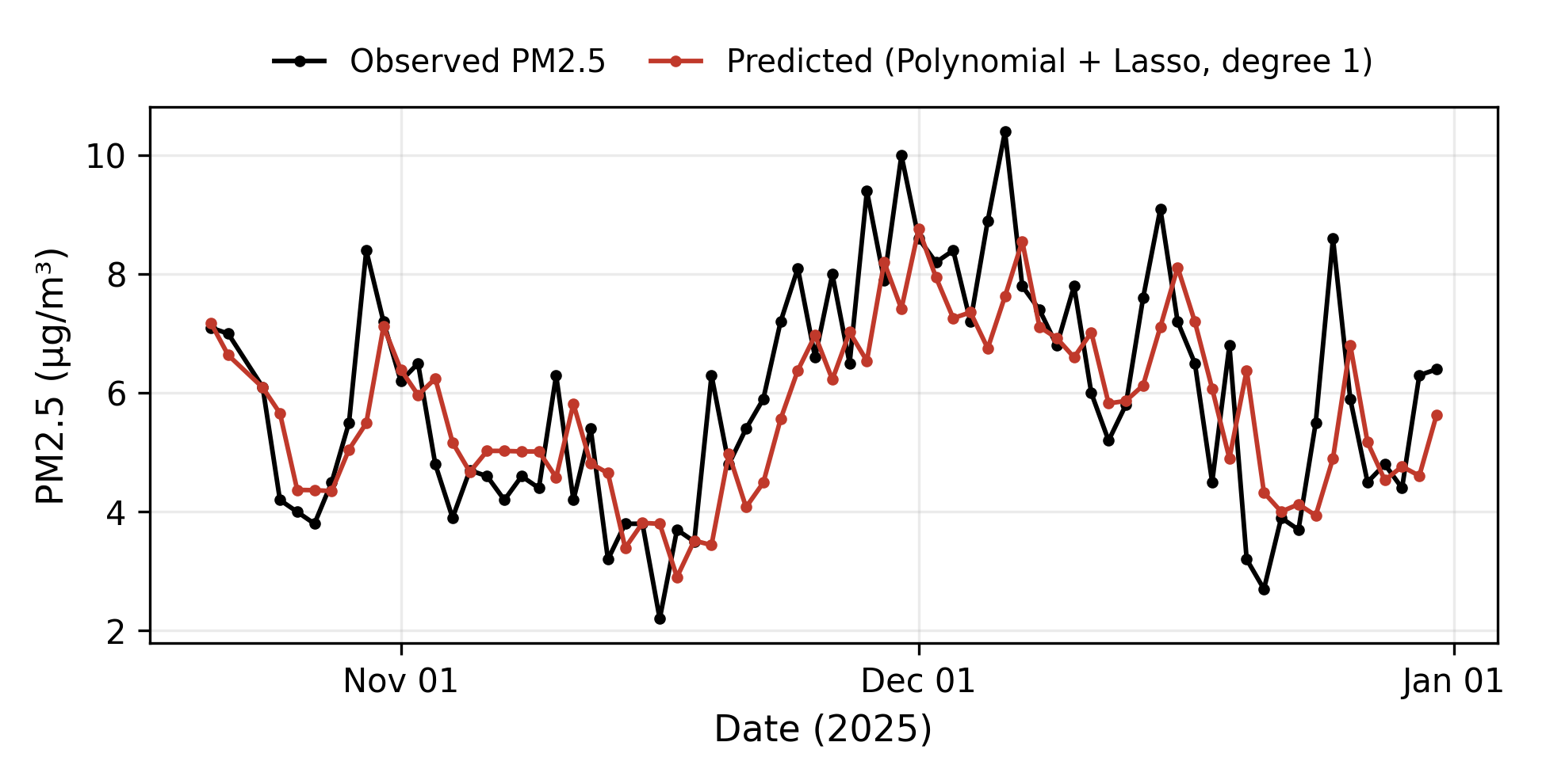
Figure 1 shows the test-period predictions following the general level and slower swings of the observed PM2.5 series, but lagging behind day-to-day spikes. This is consistent with a model whose strongest predictor is the previous day’s PM2.5 value. A persistence-dominated model is structurally prone to under-react to a sudden single-day increase and over-react to a sudden single-day decrease, since it partially carries the prior day’s level forward. This pattern is common to forecasting models that rely heavily on autoregressive structure, and is not unique to the top-performing model here. The ablation results above show that PM2.5 history alone accounts for most of the achievable R² in this dataset. That is the same underlying reason the model both performs well overall and lags at sharp transitions.

Discussion

Consistent with prior benchmarks finding that tree-based models are often competitive with or better than deep learning on tabular data^24,25, the tuned tree ensembles here outperformed the tuned neural networks, and a Lasso-regularized linear model outperformed every other model tested here. Three things should be kept separate when interpreting this ranking. First, what the results directly demonstrate: a Lasso-regularized model with no polynomial expansion generalized to the held-out test period better than the alternatives evaluated here, under this dataset size, predictor set, and evaluation design. Second, what is a plausible but unproven explanation: regularization, rather than a genuinely linear atmospheric process, may be doing much of the work. Regularized models are specifically suited to a setting with a modest sample size (282 training days) and correlated predictors. Third, what cannot be concluded from these results: that the physical relationship between weather, fire activity, vegetation, and PM2.5 is fundamentally linear. The coefficient-stability analysis (Table 6) supports the second and third points directly. Even the best-performing model’s own coefficients were not fully stable across folds, and Lasso zeroed out several fire-related predictors entirely rather than assigning them small but consistent weights.

The ablation results in Table 5 are, in the author’s view, the most important finding of this study. The weather, fire, and NDVI predictor groups were tested for their contribution to the top model’s performance, specifically whether the fire predictors contributed anything beyond prior-day PM2.5 and weather. Tested directly, using the same regularized model type and a temporally valid evaluation, fire predictors did not produce a statistically detectable improvement when added to PM2.5 history and weather. They significantly worsened a weather-only model. This does not mean wildfire smoke has no effect on PM2.5 at this site. It means that the specific fire features used here, satellite hotspot count and fire radiative power within a 100 km radius, did not translate into additional next-day predictive power beyond what prior-day PM2.5 and standard weather variables already captured, for this site and this one-year period. A defensible reading is that regional fire activity and local meteorology are themselves correlated: fires are more likely, and more likely to produce smoke impacts, under particular wind and humidity conditions that are already represented in the weather predictors. The fire features may therefore add largely redundant rather than novel information once weather is already included. Any redundant information Lasso does retain is discarded because it does not reduce cross-validated error.

The LLM few-shot approach performed the worst of any model tested (R² = −2.40). This is consistent with existing findings that LLM zero-shot and few-shot time-series forecasting is sensitive to noise and prompting choices, and does not reliably outperform purpose-built models^17,18. distilgpt2 is a small, general-purpose text model with no numerical-forecasting training and no architectural prior for atmospheric physics. This result should not be read as evidence against larger, more capable, or specifically fine-tuned language models. It is only evidence that a small, general-purpose model given five in-context examples is not currently competitive with regularized regression for this task.

This study makes no claim that measured PM2.5 at the Santa Cruz site originated from wildfire smoke specifically. The regional fire-activity predictors used here should be read as a candidate environmental covariate, not as evidence of smoke transport to the monitor. Satellite hotspot detections indicate that fire activity occurred somewhere within a defined radius. They do not by themselves establish that smoke from that activity reached the surface at a specific downwind location, a distinction documented in the smoke-transport literature^20,21. Combined with the ablation finding that fire predictors did not improve forecasts here, this study’s scope is best described as daily, site-level PM2.5 forecasting, using regional fire activity as one candidate predictor among several, rather than as wildfire-smoke forecasting.

Limitations

This study has several limitations. The dataset covers a single calendar year (2025) and a single AQS monitoring site. Findings may not generalize to other years, other Santa Cruz-area conditions, or other locations, including San Jose, the study’s originally intended target. Santa Cruz’s coastal, maritime-influenced meteorology differs from inland Central Valley or South Bay conditions, in ways that could plausibly change which predictors matter most. The final test partition contained only 71 days. This limits the precision of every reported metric and of the bootstrap confidence intervals built from it. Several of this study’s ablation and model comparisons that did not reach statistical significance might reach it with more test data. This study cannot distinguish a genuinely null effect from an underpowered one in every case.

This study does not attempt to attribute measured PM2.5 to wildfire smoke. No smoke-day classification, plume-transport model, or satellite smoke product was used. FIRMS hotspot detections indicate regional fire activity, not confirmed smoke impact at the monitoring site^20,21. HRRR weather data were sampled for only 72 of 360 days and forward-filled for the remaining days, because retrieving the full daily record was not computationally practical in the environments used for this analysis. This reduces the temporal resolution of the weather predictors relative to what the underlying HRRR product could in principle provide. NDVI’s 16-day composite structure was interpolated to daily resolution using a method that still draws on composites from both before and after a given day, rather than exclusively from prior composites. This is not fully causal, and is a limitation of the current NDVI processing: the raw sparse composite export needed to redo the interpolation as a strictly forward-looking fill was not available for this analysis.

The neural-network models (MLP, CNN) and the SARIMAX model were trained on a comparatively small sample of 282 training days. This likely limits their ability to reach their full potential, relative to what a larger multi-year dataset might support. Their weaker performance here should not be generalized to claims about these model families’ suitability for PM2.5 forecasting in general. The CNN architecture, in particular, treats an unordered feature vector as if it had sequential structure. This has no clear physical justification here, and is discussed as a limitation of the comparison rather than of CNNs generally. All model comparisons in this study reflect a single train/test split, rather than a distribution over multiple splits. Reported performance differences, beyond those directly tested with the paired bootstrap, should be interpreted with appropriate caution. Finally, this evaluation is retrospective: all data were retrieved, cleaned, and merged after the fact. This study demonstrates historical forecasting skill under a fixed forecast-origin definition, not validated operational, real-time performance, which would additionally depend on data-delivery latency for each source.

Recommendations for Future Work

Several directions follow directly from this study’s findings. Extending the dataset across multiple years and additional nearby AQS monitors would increase both training and test sample sizes. This would likely improve the neural-network and ensemble models’ ability to reach competitive performance, and narrow the bootstrap confidence intervals enough to distinguish the top regularized models from one another with more confidence. Incorporating an explicit smoke-attribution product, such as the NOAA Hazard Mapping System smoke product or a dispersion-model-based estimate, would allow a genuine test of whether wildfire smoke specifically, as opposed to regional fire activity generally, contributes to PM2.5 at this site. That is a question this study’s design cannot answer. Retrieving a complete daily HRRR record, rather than a sampled and forward-filled one, and obtaining the raw sparse NDVI composite export needed to interpolate NDVI in a strictly forward-looking, causal manner, would close two of this study’s specific data-construction limitations.

Methodologically, probabilistic or interval forecasts, rather than single-point predictions, would better communicate forecast uncertainty to a public health audience. Explicit AQI-threshold or exceedance-day classification could also be more directly actionable than a continuous PM2.5 estimate. Explainable-AI methods such as SHAP values could extend the coefficient-stability analysis performed here to the nonlinear models, which currently lack any comparable interpretability check. This study found that a Lasso-regularized linear model outperformed more complex alternatives under a leakage-audited design, while less strongly regularized linear models did not. Testing whether that finding holds at other single-site locations, or generalizes into a transferable modeling recommendation, would require replicating this analysis at additional sites, ideally including the same leakage-audit and ablation procedures used here.

Closing Thought

This study compared twelve approaches for next-day PM2.5 forecasting at a single Santa Cruz, California AQS site. Every predictor was explicitly checked against a defined forecast origin, so only information available before a given day was used to predict that day’s PM2.5. A Lasso-regularized linear model was the best-performing approach (R² = 0.478), meaningfully ahead of tuned tree ensembles, neural networks, classical time-series models, and an LLM few-shot approach. It was also statistically distinguishable from Linear Regression and Elastic Net, favoring the top model in both comparisons. A temporally valid ablation found that fire-related predictors did not significantly improve forecasts beyond prior-day PM2.5 and weather. Coefficient-stability analysis found relative humidity and the sine component of wind direction to be the most stable predictors across cross-validation folds, with PM2.5 persistence carrying the largest but less stable coefficient. These findings support a Lasso-regularized linear model as a strong, interpretable, and comparatively inexpensive baseline for site-level daily PM2.5 forecasting, and illustrate concretely how sensitive reported model accuracy can be to the details of forecast-origin alignment and feature construction.

Acknowledgement

AI-assisted tools: Portions of this project’s data analysis pipeline, code correction, and manuscript preparation were developed with the assistance of an AI language model (Anthropic’s Claude), used under the author’s direction and review at every step. All modeling decisions, interpretations, and conclusions were reviewed and approved by the author.

References

1. X. Li, X. Liu. Effects of PM2.5 on chronic airway diseases: a review of research progress. Atmosphere. Vol. 12, pg. 1068, 2021, https://doi.org/10.3390/atmos12081068. [↩]
2. S. Basith, B. Manavalan, T. H. Shin, C. B. Park, W.-S. Lee, J. Kim, G. Lee. The impact of fine particulate matter 2.5 on the cardiovascular system: a review of the invisible killer. Nanomaterials. Vol. 12, pg. 2656, 2022, https://doi.org/10.3390/nano12152656. [↩]
3. G. D. Madakumbura, M. A. Moritz, K. A. McKinnon, A. P. Williams, S. Rahimi, B. Bass, J. Norris, R. Fu, A. Hall. Anthropogenic warming drives earlier wildfire season onset in California. Science Advances. Vol. 11, pg. eadt2041, 2025, https://doi.org/10.1126/sciadv.adt2041. [↩]
4. M. Qiu, M. Kelp, S. Heft-Neal, X. Jin, C. F. Gould, D. Q. Tong, M. Burke. Evaluating chemical transport and machine learning models for wildfire smoke PM2.5. Environmental Science & Technology. Vol. 58, pg. 22880-22893, 2024, https://doi.org/10.1021/acs.est.4c05922. [↩]
5. H. Hewamalage, K. Ackermann, C. Bergmeir. Forecast evaluation for data scientists: common pitfalls and best practices. Data Mining and Knowledge Discovery. Vol. 37, pg. 788-832, 2023, https://doi.org/10.1007/s10618-022-00894-5. [↩] [↩]
6. H. Zou, T. Hastie. Regularization and variable selection via the elastic net. Journal of the Royal Statistical Society: Series B. Vol. 67, pg. 301-320, 2005, https://doi.org/10.1111/j.1467-9868.2005.00503.x. [↩] [↩]
7. C. E. Reid, M. Jerrett, M. L. Petersen, G. G. Pfister, P. E. Morefield, I. B. Tager, S. M. Raffuse, J. R. Balmes. Spatiotemporal prediction of fine particulate matter during the 2008 northern California wildfires using machine learning. Environmental Science & Technology. Vol. 49, pg. 3887-3896, 2015, https://doi.org/10.1021/es505846r. [↩]
8. Q. Di, H. Amini, L. Shi, I. Kloog, R. Silvern, J. Kelly, M. B. Sabath, C. Choirat, P. Koutrakis, A. Lyapustin, Y. Wang, L. J. Mickley, J. Schwartz. An ensemble-based model of PM2.5 concentration across the contiguous United States with high spatiotemporal resolution. Environment International. Vol. 130, pg. 104909, 2019, https://doi.org/10.1016/j.envint.2019.104909. [↩]
9. P. P. Vignesh, J. H. Jiang, P. Kishore. Predicting PM2.5 concentrations across USA using machine learning. Earth and Space Science. Vol. 10, pg. e2023EA002911, 2023, https://doi.org/10.1029/2023EA002911. [↩] [↩]
10. T. Toharudin, R. E. Caraka, I. R. Pratiwi, Y. Kim, P. U. Gio, A. D. Sakti, M. Noh, F. A. L. Nugraha, R. S. Pontoh, T. H. Putri, T. S. Azzahra, J. J. Cerelia, G. Darmawan, B. Pardamean. Boosting algorithm to handle unbalanced classification of PM2.5 concentration levels by observing meteorological parameters in Jakarta-Indonesia using AdaBoost, XGBoost, CatBoost, and LightGBM. IEEE Access. Vol. 11, pg. 35680-35696, 2023, https://doi.org/10.1109/ACCESS.2023.3265019. [↩]
11. S. K. Grange, D. C. Carslaw, A. C. Lewis, E. Boleti, C. Hueglin. Random forest meteorological normalisation models for Swiss PM10 trend analysis. Atmospheric Chemistry and Physics. Vol. 18, pg. 6223-6239, 2018, https://doi.org/10.5194/acp-18-6223-2018. [↩]
12. S. Du, T. Li, Y. Yang, S.-J. Horng. Deep air quality forecasting using hybrid deep learning framework. IEEE Transactions on Knowledge and Data Engineering. Vol. 33, pg. 2412-2424, 2021, https://doi.org/10.1109/TKDE.2019.2954510. [↩]
13. N. Zaini, L. W. Ean, A. N. Ahmed, M. A. Malek, M. F. Chow. PM2.5 forecasting for an urban area based on deep learning and decomposition method. Scientific Reports. Vol. 12, pg. 17565, 2022, https://doi.org/10.1038/s41598-022-21769-1. [↩]
14. H. Zhou, S. Zhang, J. Peng, S. Zhang, J. Li, H. Xiong, W. Zhang. Informer: beyond efficient transformer for long sequence time-series forecasting. Proceedings of the AAAI Conference on Artificial Intelligence. Vol. 35, pg. 11106-11115, 2021, https://doi.org/10.1609/aaai.v35i12.17325. [↩]
15. Y. Liang, Y. Xia, S. Ke, Y. Wang, Q. Wen, J. Zhang, Y. Zheng, R. Zimmermann. AirFormer: predicting nationwide air quality in China with transformers. Proceedings of the AAAI Conference on Artificial Intelligence. Vol. 37, pg. 14329-14337, 2023, https://doi.org/10.1609/aaai.v37i12.26676. [↩]
16. Z. Zhang, S. Zhang. Modeling air quality PM2.5 forecasting using deep sparse attention-based transformer networks. International Journal of Environmental Science and Technology. Vol. 20, pg. 13535-13550, 2023, https://doi.org/10.1007/s13762-023-04900-1. [↩]
17. N. Gruver, M. Finzi, S. Qiu, A. G. Wilson. Large language models are zero-shot time series forecasters. Advances in Neural Information Processing Systems. Vol. 36, pg. n/a, 2023, https://arxiv.org/abs/2310.07820. [↩] [↩] [↩]
18. J. Park, H. Lee, D. Lee, D. Gwak, J. Choo. Revisiting LLMs as zero-shot time-series forecasters: small noise can break large models. Proceedings of the 63rd Annual Meeting of the Association for Computational Linguistics (Volume 2: Short Papers). Vol. 2, pg. 906-922, 2025, https://aclanthology.org/2025.acl-short.71/. [↩] [↩] [↩]
19. S. Kapoor, A. Narayanan. Leakage and the reproducibility crisis in machine-learning-based science. Patterns. Vol. 4, pg. 100804, 2023, https://doi.org/10.1016/j.patter.2023.100804. [↩]
20. A. S. Kaulfus, U. Nair, D. Jaffe, S. A. Christopher, S. Goodrick. Biomass burning smoke climatology of the United States: implications for particulate matter air quality. Environmental Science & Technology. Vol. 51, pg. 11731-11741, 2017, https://doi.org/10.1021/acs.est.7b03292. [↩] [↩] [↩]
21. T. Liu, F. M. Panday, M. C. Caine, M. Kelp, D. C. Pendergrass, L. J. Mickley, E. A. Ellicott, M. E. Marlier, R. Ahmadov, E. P. James. Is the smoke aloft? Caveats regarding the use of the Hazard Mapping System (HMS) smoke product as a proxy for surface smoke presence across the United States. International Journal of Wildland Fire. Vol. 33, pg. WF23148, 2024, https://doi.org/10.1071/WF23148. [↩] [↩] [↩]
22. A. Makhdoomi, M. Sarkhosh, S. Ziaei. PM2.5 concentration prediction using machine learning algorithms: an approach to virtual monitoring stations. Scientific Reports. Vol. 15, pg. 8076, 2025, https://doi.org/10.1038/s41598-025-92019-3. [↩]
23. A. Huete, K. Didan, T. Miura, E. P. Rodriguez, X. Gao, L. G. Ferreira. Overview of the radiometric and biophysical performance of the MODIS vegetation indices. Remote Sensing of Environment. Vol. 83, pg. 195-213, 2002, https://doi.org/10.1016/S0034-4257(02)00096-2. [↩]
24. L. Grinsztajn, E. Oyallon, G. Varoquaux. Why do tree-based models still outperform deep learning on tabular data?. Advances in Neural Information Processing Systems. Vol. 35, pg. 507-520, 2022, https://arxiv.org/abs/2207.08815. [↩]
25. R. Shwartz-Ziv, A. Armon. Tabular data: deep learning is not all you need. Information Fusion. Vol. 81, pg. 84-90, 2022, https://doi.org/10.1016/j.inffus.2021.11.011. [↩]