Measuring and Shaping Gender Bias in Text Embeddings and Classifiers

Abstract

Gender bias is present in machine learning models used for tasks like sentiment analysis, hiring, and recommendations without gender as an input. This study examines two areas: gender and sentiment relationships in pre-trained text embeddings and how biased training data and classifier architectures can lead to unfair decisions. A cosine-similarity permutation test was conducted on the OpenAI text-embedding-3-large model using a synthetic corpus of 932 sentences with equal gender and nearly equal sentiment representation. A non-statistically significant (p = 0.459, 1,000 permutations), weak positive cosine similarity (0.021) was observed. Additionally, two other tests were conducted that showed similar results- a counterfactual template gender-swapping evaluation (p = 0.415) and a paraphrase robustness test (p = 0.402) which showed no statistically significant evidence of a gender-sentiment association in the embeddings. Six families of classifiers were trained on the embeddings while varying how frequently positive training examples were associated with male-coded language. Linear SVC exhibited minor bias changes as the training data became increasingly imbalanced. However, higher-capacity models like MLPClassifier and Gradient Boosting showed greater differences between demographic groups. Group-wise error analysis and threshold sensitivity testing verified these trends. The Adult Income dataset demonstrated that high accuracy can hide fairness issues. Although gender was not an input, gender-associated features conveyed gender-related information. Including race and gender increased disparity, while using a representation free of gender bias decreased disparity without reducing overall accuracy. Overall, fairness depends heavily on the training data, learned features, and classifier architecture, which can amplify or reduce gender-related disparities.

Keywords: gender fairness, text embeddings, classifier bias, NLP fairness, algorithmic fairness

Introduction

Text embeddings have been shown to represent patterns of social stereotypes including gender-related patterns in occupations¹. Caliskan et al., using the Word Embedding Association Test (WEAT), demonstrated that word embeddings trained on typical text corpora reproduce biases similar to humans². Moreover, Garg et al. demonstrated how changes in gender and ethnic stereotypes can be measured using embeddings trained on historical text collections³. It is clear that even when sensitive characteristics (e.g. gender) are removed from the input, machine learning systems may learn gender information through features associated with gender. Specifically, sentiment systems have performed differently across demographic groups⁴. Recent studies have demonstrated that pre-trained AI language models have the ability to transfer gender and other demographic biases into sentiment analysis systems across multiple groups⁵. This raises concerns that multiple subgroups will experience unfair treatment when AI analyzes subjective language.

Due to bias in embeddings, there has been much research focused on creating methods for removing bias. Bolukbasi recommended removing gender and sentiment associations from word vectors¹. However, Gonen and Goldberg indicated that this method does not remove bias but hides it while retaining its underlying form⁶. Other attempts include counterfactual data augmentation⁷, adversarial removal of protected attributes⁸, and re-weighting or constraint-based training⁹. Benchmarks such as WinoBias¹⁰ and StereoSet¹¹ serve as methods for measuring bias and evaluating model fairness across multiple dimensions. On the classification front, there are formal fairness criteria that ensure AI models do not discriminate against specific groups of people¹²¹³. Dressel and Farid showed that racial bias exists in risk assessment even with race removed¹⁴. Studies examining gender bias in contextualized embeddings have also shown that models like BERT and ELMo continue to exhibit stereotypical associations¹⁵¹⁶. Blodgett et al. surveyed 146 studies about bias in NLP and stated that much of this research did not have a clear reason why the harm was caused¹⁷. Buolamwini and Gebru pointed out intersectional accuracy disparities in commercial systems¹⁸, and Mitchell et al. proposed model cards as a way to increase transparency¹⁹. Research on bias amplification has shown that models can amplify biases present in their training data²⁰, and audits of large language models have consistently documented persistent occupational and behavioral gender stereotypes²¹.

If embeddings do align gender with sentiment, models trained on them might inherit and amplify these associations. This type of bias can go unnoticed with standard accuracy reporting. This study asks three questions: (1) Do pretrained embeddings align gender and sentiment directions beyond what would be expected by chance? (2) How does training-data imbalance interact with these associations during model learning? (3) Which model families, under the conditions tested, are most resistant to distribution disproportionalities affecting protected groups?

Answering these questions would examine how text representations, training data, and model design interact, ultimately helping fairness evaluations. In practice, models trained on data containing gender-related patterns may result in more favorable outcomes for male-coded inputs and less favorable outcomes for female-coded inputs, regardless of whether gender is used as a feature. For simplicity of analysis in this study, gender is treated as a binary category (male-coded vs. female-coded). While this approach does not include non-binary, genderqueer, or other gender identities, expanding fairness evaluations beyond the gender binary is an important direction for future research¹⁷.

This study combines a synthetic dataset composed of 932 sentences, cosine similarity permutation testing using the OpenAI text-embedding-3-large model, six classifier families trained on datasets with different amounts of data imbalance, and a real world-case study to answer these questions. This study was limited to English text, OpenAI embedding models, and binary gender categories.

Methods

The study used a controlled experimental design combining synthetic corpus experiments, directional alignment analysis of pre-trained embeddings, comparison of six classifiers under varying sampling conditions, and a real-world case study utilizing the Adult Income dataset. In the synthetic experiments, the evaluation set was held constant and only the training composition was varied. This isolated the effect of sampling imbalance. The Adult Income case study applied a similar methodology to hours per week.

Dataset Construction

The dataset was created using 932 short and synthetic sentences (572 for training and 360 for testing). The test set had equal representation across four groups: female-coded positive, female-coded negative, male-coded positive, and male-coded negative. Each sentence paired a gendered subject (girls, boys, women, or men) with a short activity phrase (e.g., “girls write code” or “boys miss baskets”).

The vocabulary of the activity phrases was varied across 215 distinct phrases rather than using a single template. This reduced the likelihood that models would learn and respond to patterns rather than the underlying sentiment. The balanced design, with equal group sizes, ruled out size as an explanation. Sampling bias was only introduced during training to create conditions where male-coded positive outcomes were either over or under-represented while evaluation remained consistent.

Three sets of analysis were used to rule out the notion that the results were influenced by the sentence templates rather than the embedding models themselves.

First, a counterfactual template-swapping evaluation was conducted. For each sentence, an equivalent version with only the gender swapped (girls to boys, women to men) while keeping all other words the same was located in the corpus, resulting in 215 matched pairs. This allows for separation of the effects of gender-related words from the sentiment expressed by the sentences.

Second, a smaller sample of 30 sentences including activity phrases (60 sentences across both genders) was created. For them, two to three paraphrased versions were generated expressing the same sentiment using different vocabulary and sentence structures. Third, 30 gender-neutral sentences without gendered pronouns or names (e.g., “The student completed the assignment on time”) were added as controls. All data and code are available at: https://github.com/SaanikaGW/Embedding-CosineSimilarity-Classifier-AdulData²².

Embeddings

One pre-trained OpenAI text embedding model was used to generate sentence embeddings: text-embedding-3-large (3,072 dimensions)²³²⁴. This model was used in embedding alignment analysis and classifier experiments. The embedding weights were held constant throughout all experiments; fine-tuning was not done.

Classifiers

Six classifier families were evaluated to see how model architecture influenced bias. Logistic Regression creates a straight-line decision boundary for classifying data and converts the data into probability estimates for each class using the sigmoid function (L2 regularization, C=1.0). Linear Regression estimates a continuous value that was truncated at values of 0 and 1 to remove extreme outliers and then classified using a threshold of 0.5. Unlike Logistic Regression, however, these values are not measured as probabilities. Support Vector Classifier draws the widest possible straight line with a linear kernel to separate two groups while allowing a few mistakes controlled by a setting called C which equals 1.0. Random Forest makes a final prediction by combining the guesses of one hundred smaller decision trees trained on mixed information. Gradient Boosting also uses 100 trees. However, each tree is built sequentially to correct errors made by previous trees (learning rate=0.1, max depth=3). The MLPClassifier is a simple neural network with one hidden layer containing 100 neurons, ReLU activation, Adam optimizer, and a learning rate of 0.001, with a maximum of 200 iterations. All other hyperparameters were left at their default values from scikit-learn (version 1.3)²⁵ so that differences in performance would mainly be due to architectural distinctions among models rather than extensive tuning. A fixed random seed of 42 was used throughout.

Classifier	Configuration
Logistic Regression	Linear decision boundary, sigmoid output; C = 1.0, L2 penalty
Linear Regression	Continuous prediction clipped to [0,1]; threshold 0.5 for labels (not inherently calibrated)
Linear SVC	Maximum-margin separating hyperplane, linear kernel; C = 1.0
Random Forest	Bagged ensemble of 100 decision trees on random feature/sample subsets (sklearn defaults)
Gradient Boosting	Sequential ensemble of 100 trees correcting prior residuals; learning rate = 0.1, max depth = 3
MLPClassifier	Single hidden layer of 100 units, ReLU; Adam, learning rate = 0.001, max 200 iterations

Directional Alignment Analysis

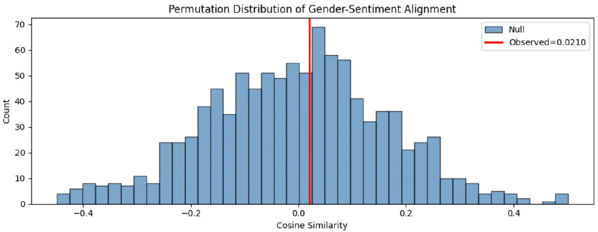
In order to assess whether there is a correlation between the gender-sentiment relationships that are captured by embeddings, the mean embedding vectors of the positively labeled sentences (μ_pos) and negatively labeled sentences (μ_neg) were calculated, as well as those of the female-coded sentences (μ_f) and male-coded sentences (μ_m). Two directional vectors were constructed from these means: v_s = μ_pos – μ_neg and a gender directional vector v_g = μ_f – μ_m. The cosine similarity between these two vectors was then computed. A high cosine similarity indicated that the embedding space linked gender with sentiment. Gender labels were randomly given 1,000 times to assess whether the result exceeded what would be expected by random chance. After each permutation the cosine similarity was re-calculated which produced a null distribution. The p-value was calculated as the proportion of permuted results that were equal to or exceeded the observed value. This procedure was repeated for the counterfactual (template-swapped) sentence set and the paraphrase sentence set.

Finally, a bootstrap stability analysis was conducted by re-sampling 80% of sentences 500 times and conducting alignment for each resample. There are also other ways to test for bias including WEAT², WinoBias¹⁰ and StereoSet¹¹.

Bias Metric and Controlled Sampling

Bias can be thought of as the average difference in predicted scores (for male-associated sentences) from those (for female-associated sentences) of the positive and negative test cases. Parameter p specifies what percentage of the positive training examples are given to the male-associated sentences. When p=0.5, positive examples are divided equally. At extreme values (p=0 or p=1), all positive training examples belong solely to one of the gender categories. Since the test set never changes, any change in bias comes from the training mix. Each sampled training set contained 276 sentences, 138 per gender, while the 360-sentence test set stayed the same.

In addition to the mean prediction gap, group-wise accuracy (male-coded positive, male-coded negative, female-coded positive, female-coded negative) and group-wise error rates are presented at key checkpoints (p=0.0, 0.25, 0.5, 0.75, 1.0).

Real Data Validation

The UCI Adult Income dataset²⁶, a well-known benchmark in fairness research^12,13, was used to assess whether a similar pattern develops in real-world socioeconomic data. The Logistic Regression models were trained using three sets of features. Further, a debiased “hours-per-week” variable was created (formula: debiased_hours_i = hours_i + (mean_hours_male – mean_hours_female) × 1(female_i)). Men in the dataset work an average of 42.4 hours per week, women 36.4. This added six hours to each female record. This method ensures that all groups have the same means but the variances within the group remain intact.

While there exist more advanced methods such as regressing out hours with respect to gender or adversarial debiasing⁸, results are reported as mean bias along with standard deviations across ten random 80/20 train-test splits. To aid in evaluating model accuracy, a majority-class baseline (predicting ≤50K for all individuals), achieving approximately 75.9% accuracy was conducted. Lastly group-wise classification and error rates along with mean prediction gaps were reported.

Results

Embedding Structure: Baseline Check

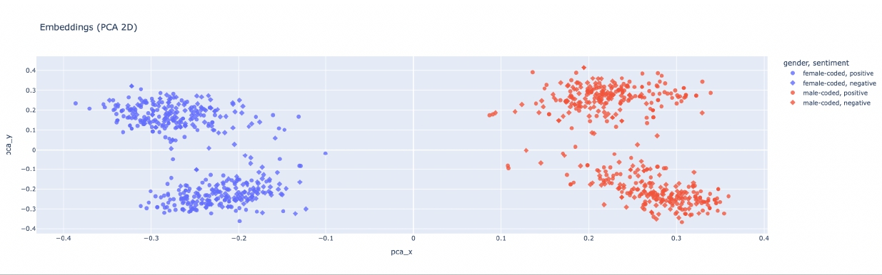
As a preliminary evaluation, a PCA plot of text-embedding-3-large vectors demonstrated that sentences mainly group by gender. Sentiment constitutes a secondary grouping. A straightforward linear model can accurately predict a sentence’s gender from these embeddings with almost perfect accuracy. Given that text contains explicit gendered words, this ability to recover is expected and does not necessarily imply that embedding models have an unfair underlying structure. The tests below check whether the pattern survives when structure and vocabulary are held constant.

Alignment Analysis Across Models

Permutation testing revealed that cosine similarity between gender and sentiment direction vectors was not statistically significant. Testing text-embedding-3-large, observed cosine similarity was 0.0210. This value lies squarely within our random baseline (permutation null mean = -0.0039, SD = 0.1673). It thus falls within the 95% range of the null distribution [-0.3539, 0.3224] and fails to meet the statistical significance criteria (p = 0.459) vs. (alpha = 0.05). To confirm this, a bootstrap resampling routine was conducted with 500 iterations and 80% subsampling. The subsequent mean alignment of 0.0214 (SD = 0.0406) and its 95% confidence interval [-0.0637, 0.0965] confirmed that the original result sits inside the range expected by chance. The upward drift is not reliable because zero is in the interval and only 72.2% of samples trended positive.

The counterfactual template-swapping analysis identified 215 matched sentence pairs (cosine similarity between matched pairs: mean = 0.7994, SD = 0.0428). When only gender terms were swapped while holding templates constant, the observed alignment was 0.029 with a permutation p-value of 0.415, again not reaching statistical significance. Gender-neutral control sentences (created by averaging male and female embeddings for each template) retained strong sentiment classification accuracy (5-fold CV: 98.6%, SD = 0.011), indicating that sentiment structure largely survives gender removal. The low alignment score of -0.209 shows that the neutralization process did not accidentally link gender to sentiment. New gender-neutral sentences achieved 100% sentiment accuracy. A gender classifier trained on the original data categorized all 30 sentences identically. While this suggests minimal gender bias in truly neutral text, it may also indicate that the classifier struggled to process text stripped of gender markers.

An analysis of 216 paraphrased variants, with 60 original sentences and 156 paraphrases consistently resulted in non-significant results. Across all of the groupings the similarity and p-values remained statistically insignificant. No significant differences were found for the original sentences alone (sim = 0.061, p = 0.408), the paraphrased versions alone (sim = 0.049, p = 0.424), or all data combined (sim = 0.053, p = 0.402). Even when all the data are taken together the result is the same (sim = 0.053, p = 0.402). Such consistency in the validation process shows that the lack of alignment is not some obvious artifact of the template structure but a genuine finding.

Sampling-Driven Classifier Bias

The bias curves illustrate that various model families respond uniquely to modifications in training data. Specifically: Linear SVC was minimally affected by changes to the training data. MLPClassifier and Gradient Boosting showed large increases in bias as the proportion of positive examples varied. Logistic Regression, Linear Regression, and Random Forest showed moderate sensitivity.

Despite gender not serving as an input feature, models still learned gender-related information from embeddings.

Classifier	p = 0.0	p = 0.25	p = 0.5	p = 0.75	p = 1.0	Acc. at p = 0.5
Logistic Regression	−0.665	−0.255	−0.007	+0.241	+0.668	0.986
Linear Regression	−0.783	−0.003	+0.012	+0.029	+0.819	0.978
Linear SVC	−0.408	−0.057	−0.011	+0.078	+0.414	0.983
Random Forest	−0.611	−0.249	−0.019	+0.230	+0.638	0.964
Gradient Boosting	−0.828	−0.238	−0.017	+0.174	+0.800	0.939
MLPClassifier	−0.957	−0.054	−0.002	+0.047	+0.962	0.983

At extreme values (p = 0.0 and p = 1.0), female-coded positive sentences are considerably more likely to be misclassified as negative when most positive training examples are male-coded. Similarly, male-coded negative sentences are more likely to be erroneously classified as positive. This pattern, and its mirror image at p = 0.0, appeared for all six classifiers. Every classifier except Gradient Boosting misclassified 100% of these sentences and Gradient Boosting misclassified 81-98%.

For three models generating probability outputs (Logistic Regression, Gradient Boosting, MLPClassifier), changing the decision threshold from 0.3 to 0.7 at p = 0.5 had no effect on bias. This was because the bias metric uses predicted scores rather than thresholded labels. Threshold changes affected accuracy instead. It was the most for Logistic Regression (0.772 to 0.969) and least for MLPClassifier (0.969 to 0.975).

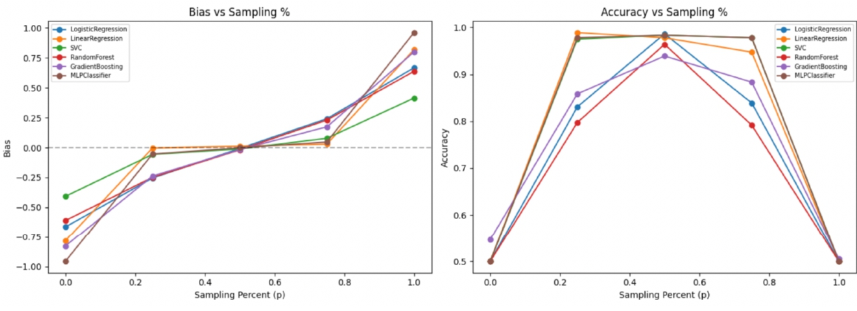
Linear SVC tends to be quite consistent in its behavior under different sampling conditions when run with the default hyperparameters. Logistic Regression and Linear Regression were less stable. Also, Linear Regression reached bias levels close to Gradient Boosting at the extremes. On the other hand, higher-capacity approaches (such as Gradient Boosting or the MLPClassifier) magnify disparity where there are extreme skews. This results in steeper slopes and larger swings in bias.

Changes in hyperparameter configuration (e.g., a lower learning rate, fewer trees or more aggressive regularization) can change that dynamic. Hence, fairness metrics should be considered and weighted alongside accuracy when hyperparameters are selected.

Real-Data Vignette: Social Correlation Drives Downstream Bias

The synthetic experiments have made it clear that the interplay of sampling and gender-sentiment links can give rise to gender disparities, gender being an explicit feature or not. The study now puts a similar mechanism to the test in an actual socioeconomic context with the Adult Income dataset.

Take the matter of hours worked: in the Adult dataset, men put in more time on average than women (some 42.4 hours a week as against 36.4). Since there is a strong link between longer hours and higher pay, a model will pick up on these gendered differences through its inputs even if one has left gender out of the feature set. For reference, a majority-class baseline, simply predicting the most common income class for everyone, comes in at about 75.9 per cent accuracy. The figures below are to be viewed in light of that.

Consider a model with hours per week as its sole feature, gender excluded. It will hand men higher income probabilities on account of their greater average working hours. The mean score for men is thus higher than for women (a bias of +0.048 ± 0.002 over 10 splits), yet at 0.754 ± 0.005 the accuracy is only marginally better than the majority-class floor. One can see that while the feature’s correlation with gender leads to disparate outcomes, hours alone do not offer much in the way of predictive power over and above class imbalance.

When race and gender are added as explicit features to the mix, the model has access to the direct label as well as the indirect signal from hours. This increases the disparity in predicted scores to a bias of +0.196 ± 0.002. However, accuracy is barely affected. There is a widening inequity while the average outcomes remain unchanged.

The study also looks at the impact of changing the hours per week. This is done by increasing female observations up by the roughly six-hour gap gap (i.e., debiased_hours_i = hours_i + (mean_hours_male – mean_hours_female) × 1(female_i)). The result is a near parity in mean predicted scores for the two sexes (bias = 0.000 ± 0.001) with no loss to the overall accuracy of 0.756 ± 0.005.

Feature configuration	Mean bias (M − F)	Accuracy	% predicted high-income (M / F)
Hours per week only	+0.048 ± 0.002	0.754 ± 0.005	3.2% / 1.2%
Race + gender + hours/week	+0.196 ± 0.002	0.756 ± 0.004	4.1% / 0.2%
Debiased hours per week	0.000 ± 0.001	0.756 ± 0.005	1.7% / 1.2%

When one looks at the group-wise classification rates for the hours-only model, 3.2% of men are put in the high-income category at a 0.5 threshold compared to 1.2% of women. Introduce race and gender as additional features and that disparity widens, with 4.1% of men predicted as high income against just 0.2% of women. Debiasing serves to close the gap. This narrowed, but didn’t close the gap, with the figures then being 1.7% for men and 1.2% for women.

What is seen in the Adult Income data is much like the mechanism at play in our synthetic experiments. Even in the absence of an explicit gender variable, features that hold gender information can lead to disparate predictions, and a change in representation will see the disparity diminish. Yet there are some important differences between the two. The synthetic corpus is a controlled environment with a clean setup where the origin of the gender data is unambiguous. The Adult data, by contrast, has the confounds of the real world. Hours worked are tied to occupation and education as well as gender. While the debiasing process in the synthetic work is a matter of adjusting embeddings, here it is applied to a single tabular feature. So, while the Adult example illustrates the same principle, it cannot be interpreted to say that the mechanisms are identical.

Discussion

There are three key findings. First, there was no statistically significant evidence supporting a gender-sentiment relationship in embeddings: observed cosine similarity fell within the range of expected variation. Counterfactual template-swapping and paraphrase robustness tests showed similar results. In the 932-sentence corpus using OpenAI embeddings there was little evidence of gender-sentiment alignment beyond chance.

Second, imbalanced training data produced substantial bias in classifiers despite gender not being an input feature. As the proportion of positive examples moved towards one gender, classifier predictions shifted, with the magnitude depending on the model family.

Third, under tested conditions, Linear SVC showed the least impact to sampling skew whereas MLPClassifier and Gradient Boosting had the greatest bias. Logistic Regression, Linear Regression, and Random Forest fell somewhere in-between. The ranking may differ based on hyperparameters employed.

Ultimately, results demonstrate that at least in this study, bias came not from embeddings but from a combination of gender-correlated training data (or features similar to the Adult Income example) and model capacity. Even though overall accuracy stayed high, prediction gaps between groups expanded under skewed training conditions. Embedding audits, controlled sampling, and fairness-focused evaluation can help AI developers identify where bias enters systems used for high-stakes decisions, including hiring, lending, and education, before those biases affect real people.

Using default hyperparameters, models with higher capacity (e.g., MLPClassifier and Gradient Boosting) were more sensitive to sampling skew. This was unlike models like Linear SVC, which was least affected, Logistic Regression, Linear Regression and Random Forest. It is unclear if this pattern applies to other datasets, embedding types and hyperparameter configurations. Hence, when fairness is important, developers should assess fairness metrics in addition to accuracy metrics.

The debiasing method used in this study (i.e., a simple mean-shift applied to the Adult data) was intentionally kept simple to show that changing a gender-related feature can lessen disparities. More sophisticated methods include projection-based debiasing¹, counterfactual data augmentation⁷ and re-weighting⁹²⁷. For genuine fairness issues, established techniques should be considered. Integrating embedding audits, sampling sweeps and real-data examples are a feasible starting point for fairness analysis.

Researchers should further question which models are sensitive to biased sampling other than just evaluating accuracy metrics. Additionally, they can assess features that convey protected group information and interventions that best reduce inequalities. To turn this into a generalized framework, it should be applied to additional tasks, datasets and embedding types. The main contribution of this work lies in demonstrating how these three diagnostic methods can be used together. Auditing embeddings, testing different data groups, and looking at real examples is a practical way to start testing for fairness.

Ethical Considerations

This study did not involve human participants or private data and instead relied on synthetic sentences or publicly available datasets.

Choosing to ‘debias’ a feature like hours-worked assumes that gender differences in hours worked are partially caused by structural inequality and that making this equal in the model is an appropriate course of action. In other cases, group differences may represent legitimate variations that should not be removed. Determining what constitutes “bias” versus “signal” requires knowledge from field experts and input from affected communities¹⁷. Further, there exists a potential risk that debiasing could happen superficially solely for the sake of satisfying fairness requirements without addressing underlying causes of inequality. Fairness interventions can create unexpected outcomes if not carefully considered within their respective contexts.

The study treats gender as binary. Therefore, non-binary, genderqueer and other identities are not encompassed. Expanding fairness analysis to include these groups represents an important avenue for future research.

Limitations

The study has several limitations.

The synthetic corpus contains only 932 sentences and limited vocabulary written by one person. Inter-annotator reliability was not verified. Therefore, subtle associations between gender and writing style cannot be excluded although counterfactual and paraphrase checks help reduce this risk. Only OpenAI embedding models were tested. Testing open-source embeddings such as Sentence-BERT or GloVe would support arguments about embedding bias in general.

Further, classifier experiments using default hyperparameters and alternative settings might show different patterns. The bias metric (i.e., mean prediction gap) assesses only one aspect of fairness and other metrics like equalized odds, calibration and individual fairness were not thoroughly examined. The Adult Income example uses one feature and a simple debiasing method. Actual applications would require more detailed feature analysis and complex interventions²⁸.

Lastly, the study focuses solely on English text and binary gender, limiting its use in other languages and gender identities. Future research may extend this analysis to larger datasets, more tasks, current embeddings and non-binary representations of gender.

Conclusion

To summarize, the study addressed three basic questions.

First, there was no statistically significant evidence suggesting that pre-trained embeddings link gender with sentiment beyond what would happen randomly. Observed cosine similarity was not greater than the value obtained from the permutation null hypothesis. Counterfactual template-swapping and paraphrase robustness checks showed similar results. There was little evidence showing gender-sentiment alignment beyond chance in the 932-sentence corpus using OpenAI embeddings.

Second, imbalanced training data produced clear, substantial bias in classifiers despite gender not being an input feature. As the proportion of positive examples moved towards one gender, classifier predictions shifted, with the extent depending on model family.

Third, Linear SVC was most resistant to sampling skew while MLPClassifier and Gradient Boosting showed greatest bias.

Overall, results indicate that at least in this study, bias came not from embeddings but from a mixture of gender-correlated training data (or features similar to the Adult Income example) and model capacity.

Although overall accuracy was high, the differences between groups grew when the training data was unbalanced. Embedding audits, balanced sampling, and fairness testing can help identify and reduce bias when building models for sensitive applications. As machine-learning systems are increasingly used in hiring, lending, and education, considering not only the extent of bias but when it occurs in the process is also crucial.

Acknowledgments

The author thanks Tyler Giallanza for his mentorship and continued guidance.

References

1. T. Bolukbasi, K.-W. Chang, J. Y. Zou, V. Saligrama, A. T. Kalai. Man is to computer programmer as woman is to homemaker? Debiasing word embeddings. Advances in Neural Information Processing Systems. Vol. 29, pg. 4349-4357, 2016. [↩] [↩] [↩]
2. A. Caliskan, J. J. Bryson, A. Narayanan. Semantics derived automatically from language corpora contain human-like biases. Science. Vol. 356, No. 6334, pg. 183-186, 2017, https://doi.org/10.1126/science.aal4230. [↩] [↩]
3. N. Garg, L. Schiebinger, D. Jurafsky, J. Zou. Word embeddings quantify 100 years of gender and ethnic stereotypes. Proceedings of the National Academy of Sciences. Vol. 115, No. 16, pg. E3635-E3644, 2018, https://doi.org/10.1073/pnas.1720347115. [↩]
4. S. Kiritchenko, S. M. Mohammad. Examining gender and race bias in two hundred sentiment analysis systems. Proceedings of the Seventh Joint Conference on Lexical and Computational Semantics (*SEM). pg. 43-53, 2018, https://doi.org/10.18653/v1/S18-2005. [↩]
5. K. Mei, S. Fereidooni, A. Caliskan. Bias against 93 stigmatized groups in masked language models and downstream sentiment classification tasks. Proceedings of the 2023 ACM Conference on Fairness, Accountability, and Transparency. pg. 1699-1710, 2023, https://doi.org/10.1145/3593013.3594109. [↩]
6. H. Gonen, Y. Goldberg. Lipstick on a pig: Debiasing methods cover up systematic gender biases in word embeddings but do not remove them. Proceedings of the 2019 Conference of the North American Chapter of the Association for Computational Linguistics: Human Language Technologies (NAACL-HLT), Vol. 1. pg. 609-614, 2019, https://doi.org/10.18653/v1/N19-1061. [↩]
7. R. Zmigrod, S. J. Mielke, H. Wallach, R. Cotterell. Counterfactual data augmentation for mitigating gender stereotypes in languages with rich morphology. Proceedings of the 57th Annual Meeting of ACL. pg. 1651-1661, 2019, https://doi.org/10.18653/v1/P19-1161. [↩] [↩]
8. B. H. Zhang, B. Lemoine, M. Mitchell. Mitigating unwanted biases with adversarial learning. Proceedings of the 2018 AAAI/ACM Conference on AI, Ethics, and Society. pg. 335-340, 2018, https://doi.org/10.1145/3278721.3278779. [↩] [↩]
9. A. Agarwal, A. Beygelzimer, M. Dudík, J. Langford, H. Wallach. A reductions approach to fair classification. Proceedings of the 35th ICML (PMLR Vol. 80). pg. 60-69, 2018. [↩] [↩]
10. J. Zhao, T. Wang, M. Yatskar, V. Ordonez, K.-W. Chang. Gender bias in coreference resolution: Evaluation and debiasing methods. Proceedings of NAACL-HLT. pg. 15-20, 2018, https://doi.org/10.18653/v1/N18-2003. [↩] [↩]
11. M. Nadeem, A. Bethke, S. Reddy. StereoSet: Measuring stereotypical bias in pretrained language models. Proceedings of the 59th Annual Meeting of ACL. pg. 5356-5371, 2021, https://doi.org/10.18653/v1/2021.acl-long.416. [↩] [↩]
12. M. Hardt, E. Price, N. Srebro. Equality of opportunity in supervised learning. Proceedings of the 30th International Conference on Neural Information Processing Systems (NeurIPS). pg. 3315-3323, 2016. [↩] [↩]
13. S. Barocas, A. D. Selbst. Big data’s disparate impact. California Law Review. Vol. 104, pg. 671-732, 2016. [↩] [↩]
14. J. Dressel, H. Farid. The accuracy, fairness, and limits of predicting recidivism. Science Advances. Vol. 4, No. 1, eaao5580, 2018, https://doi.org/10.1126/sciadv.aao5580. [↩]
15. C. Basta, M. R. Costa-jussà, B. Casas. Evaluating the underlying gender bias in contextualized word embeddings. Proceedings of the 1st Workshop on Gender Bias in Natural Language Processing. pg. 33-39, 2019, https://doi.org/10.18653/v1/W19-3805. [↩]
16. K. Kurita, N. Vyas, A. Pareek, A. W. Black, Y. Tsvetkov. Measuring bias in contextualized word representations. Proceedings of the 1st Workshop on Gender Bias in Natural Language Processing. pg. 166-172, 2019, https://doi.org/10.18653/v1/W19-3823. [↩]
17. S. L. Blodgett, S. Barocas, H. Daumé III, H. Wallach. Language (technology) is power: A critical survey of “bias” in NLP. Proceedings of the 58th Annual Meeting of ACL. pg. 5454-5476, 2020, https://doi.org/10.18653/v1/2020.acl-main.485. [↩] [↩] [↩]
18. J. Buolamwini, T. Gebru. Gender shades: Intersectional accuracy disparities in commercial gender classification. Proceedings of the 1st Conference on Fairness, Accountability and Transparency (PMLR). Vol. 81, pg. 77-91, 2018. [↩]
19. M. Mitchell, S. Wu, A. Zaldivar, P. Barnes, L. Vasserman, B. Hutchinson, E. Spitzer, I. D. Raji, T. Gebru. Model cards for model reporting. Proceedings of the Conference on Fairness, Accountability, and Transparency. pg. 220-229, 2019, https://doi.org/10.1145/3287560.3287596. [↩]
20. M. Hall, L. van der Maaten, L. Gustafson, M. Jones, A. Adcock. A systematic study of bias amplification. arXiv preprint arXiv:2201.11706, 2022, https://arxiv.org/abs/2201.11706. [↩]
21. H. Kotek, R. Dockum, D. Q. Sun. Gender bias and stereotypes in Large Language Models. Proceedings of The ACM Collective Intelligence Conference (CI ’23). pg. 12-24, 2023, https://doi.org/10.1145/3582269.3615599. [↩]
22. S. Dutta. Embedding-CosineSimilarity-Classifier-AdulData (GitHub repository). https://github.com/SaanikaGW/Embedding-CosineSimilarity-Classifier-AdulData, 2025. [↩]
23. OpenAI. New embedding models and API updates. OpenAI, January 25, 2024, https://openai.com/index/new-embedding-models-and-api-updates/. [↩]
24. A. Neelakantan, T. Xu, R. Puri, A. Radford, J. M. Han, J. Tworek, et al. Text and code embeddings by contrastive pre-training. arXiv preprint arXiv:2201.10005, 2022, https://arxiv.org/abs/2201.10005. [↩]
25. F. Pedregosa, G. Varoquaux, A. Gramfort, V. Michel, B. Thirion, et al. Scikit-learn: Machine learning in Python. Journal of Machine Learning Research. Vol. 12, pg. 2825-2830, 2011. [↩]
26. B. Becker, R. Kohavi. Adult [Dataset]. UCI Machine Learning Repository, 1996, https://doi.org/10.24432/C5XW20. [↩]
27. F. Calmon, D. Wei, B. Vinzamuri, K. N. Ramamurthy, K. R. Varshney. Optimized pre-processing for discrimination prevention. Proceedings of the 31st NeurIPS. pg. 3992-4001, 2017. [↩]
28. T. Schick, S. Udupa, H. Schütze. Self-diagnosis and self-debiasing: A proposal for reducing corpus-based bias in NLP. Transactions of the Association for Computational Linguistics. Vol. 9, pg. 1408-1424, 2021, https://doi.org/10.1162/tacl_a_00434. [↩]