Storage Conditions Improve Deep Learning Prediction of Remaining Avocado Shelf-Life

Abstract

Post-harvest food loss is substantial, and a large share of it occurs at the retail and consumer stages. Deep learning can estimate fruit ripeness from photographs, but existing models treat ripening as though it proceeds at a fixed rate, ignoring its well-established dependence on storage conditions. This study quantifies how much predictive accuracy a convolutional neural network gains from being told a fruit’s storage condition alongside its image, and isolates which aspect of that condition carries the gain. Using a public dataset of 14,710 photographs of 478 individually tracked ‘Hass’ avocados stored under refrigerated, ambient, and warm conditions and photographed daily until the end of shelf-life, we derived measured days-remaining labels and trained ResNet-18 regression models across eight input configurations under repeated grouped cross-validation. Data were split at the level of individual fruit to prevent leakage; predictions were aggregated per fruit and confidence intervals obtained by bootstrapping fruit rather than photographs. Supplying storage condition reduced fruit-weighted mean absolute error from 1.66 to 1.13 days, a 32% improvement (95% CI [0.46, 0.61] days, excluding zero). Zero-valued and permuted-environment controls with identical network capacity produced no improvement, showing the gain reflects genuine environmental information rather than added model parameters. A continuous temperature value did not outperform a three-level categorical storage indicator, so across these three regimes the improvement is attributable to storage condition rather than to temperature as a continuous physical variable. Photographs reveal a fruit’s state; knowing its storage condition reveals how fast that state is changing.

Keywords: Deep Learning, Convolutional Neural Networks, Transfer Learning, Multi-Modal Fusion, Ablation Study, Post-Harvest Technology, Shelf-Life Prediction, Ripeness Estimation, Regression, Food Waste, Persea americana, ResNet-18.

Introduction

Background and Context

Reducing post-harvest loss is one of the more tractable levers available for improving food system efficiency. Losses accumulate across the supply chain, but a substantial share occurs at the retail and consumer stages, where fruit is discarded either because it has spoiled unnoticed or because it is thrown away pre-emptively when its condition is uncertain. A consumer holding an avocado has no reliable way to answer a simple and consequential question: how many days remain before this fruit reaches, and then passes, its peak?

Computer vision offers a plausible route to answering that question from a single photograph. Since deep convolutional neural networks (CNNs) demonstrated their capability on large-scale image classification^1,2, they have been applied extensively to agricultural produce. A recent survey of the field³ documents a large and rapidly growing body of work on fruit ripeness classification, and concludes that pretrained-and-finetuned deep models are the most promising approach; the architectures it reviews are predominantly ImageNet-pretrained backbones such as ResNet⁴, VGG and MobileNet. Reported accuracies on curated datasets are frequently high, commonly falling between 80% and 100%, and comparable results have been obtained with classical feature-based approaches for individual species — 97.75% for banana ripeness using hand-engineered colour, spot and texture features⁵.

That maturity is itself a problem for new work. Discrete ripeness-stage classification — sorting an image into “unripe,” “ripe,” or “overripe” — is close to saturated, and a further demonstration of it adds little. Several groups have accordingly moved to the harder and more useful framing of estimating time remaining rather than current category. Davur et al. trained a spectral–spatial residual network on 551 hyperspectral images of 80 Hass avocados and predicted days-to-ripeness with a mean error of 1.17 days⁶. Jada et al. compared classification against regression for banana shelf-life using MobileNetV2 on ordinary RGB images and reported a regression mean absolute error (MAE) of 1.44 days⁷.

Problem Statement and Rationale

A limitation runs through this regression literature. These models take an image as their sole input and, in doing so, implicitly assume that ripening advances at a fixed rate. Post-harvest science says otherwise, and has said so for decades. Chen and Ramaswamy showed that colour and texture change in ripening fruit follows kinetics whose rate constants are well described by the Arrhenius equation, meaning ripening rate varies systematically and steeply with temperature⁸. The same temperature dependence is documented specifically for avocado: respiration rises with temperature across the physiological range⁹; firmness and colour have been modelled with Arrhenius rate constants fitted across multiple storage temperatures^10,11; and the daily ripening rate itself increases with storage temperature¹². An image captures a fruit’s present condition; it does not, on its face, disclose the thermal environment that will govern how quickly that condition changes.

The obvious remedy is to give the model temperature information as well. Multi-modal fusion is itself well established¹³: Liu et al. fused colour imaging with visible/near-infrared spectroscopy and haptic firmness for tomato maturity, improving accuracy from 94.2% using imaging alone to 99.4% when fused¹⁴. Yang et al. combined RGB images with greenhouse time-series environmental data through a late-fusion architecture to predict optimal melon harvest date¹⁵. Smartphone imaging has likewise been combined with multiple ripening temperatures to estimate banana quality indices, although through hand-crafted colour features rather than learned representations¹⁶.

A gap runs through this fusion literature. These studies report that a fused model outperforms a single-modality one, but the modalities being compared usually differ in more than one input at once, and the environmental branch adds parameters as well as information — so a fused model may improve partly because it is simply larger. As a result, how much the environmental context contributes on its own, and which environmental variable carries that contribution, has not to our knowledge been isolated in a controlled ablation on a days-remaining target. When a fruit’s storage condition can be summarised by its temperature, its humidity, or simply a label of which regime it was kept in, these are usually bundled into one input vector, leaving open which of them the model actually exploits.

That distinction matters both scientifically and practically. Scientifically, attributing a gain to “temperature” implies the model has learned the physical temperature-dependence of ripening, whereas a categorical label of the storage regime would imply only that it has learned to distinguish a few discrete conditions. Practically, if the environmental context contributes little beyond what appearance already reveals, a photograph-only application is sufficient and simpler; if it contributes substantially, a deployed system must capture it, and how it must capture it — a precise temperature or merely a category — determines the engineering.

Significance and Purpose

This study measures that contribution directly. We use a dataset uniquely suited to the question: 478 individual ‘Hass’ avocados, each tracked and photographed daily from three days post-harvest until the end of its shelf-life, distributed across three controlled storage environments¹⁷. Because each fruit is followed individually with timestamps, the days-remaining label is measured rather than assumed — a meaningful methodological improvement over prior RGB work, which derived day labels from stage class names under a temperature-blind constant⁷. The three storage groups are genuine experimental treatments, though only two of them have fully documented environmental conditions — a limitation addressed directly in the Methods and in a dedicated sensitivity analysis.

Objectives

1. Establish non-learned baselines that any learned model must beat, and measure how much storage condition alone predicts without any image.
2. Compare eight input configurations under identical fruit folds and an identical image branch, including zero-valued and permuted-environment controls, to isolate the marginal contribution of the environmental channel from the capacity its branch adds.
3. Determine whether that contribution is carried by a continuous temperature value or merely by a categorical indicator of the storage regime.
4. Determine whether appearance alone already encodes storage condition, by training a separate classifier to predict storage group from images, and use the result to interpret the per-group pattern.
5. Test how sensitive the result is to the one storage condition whose temperature was not precisely recorded.

Scope and Limitations

The study is confined to a single cultivar (‘Hass’ avocado) and a single dataset collected under laboratory-controlled storage. We predict days until the documented end of shelf-life, not consumer preference or internal quality attributes such as firmness or oil content. Development of any consumer-facing application is outside this scope. Limitations arising from right-censoring, incomplete environmental documentation, and class imbalance are addressed in the Discussion.

Methods

Dataset

We used the publicly available ‘Hass’ Avocado Ripening Photographic Dataset, released under a Creative Commons Attribution 4.0 licence¹⁷. It comprises 14,710 labelled JPEG photographs at 800 × 800 pixels of 478 Hass avocados (Persea americana Mill. cv Hass), acquired three days post-harvest.

Fruit were allocated to three storage groups: T10 (10 °C, 85% relative humidity), T20 (20 °C, 85% RH), and Tamb (ambient laboratory conditions). Each fruit was photographed daily, twice per session from opposite sides, and each photograph was assigned a stage on a five-point Ripening Index: 1 Underripe, 2 Breaking, 3 Ripe (First Stage), 4 Ripe (Second Stage), 5 Overripe. Stage 4 is documented as marking the end of shelf-life. An accompanying spreadsheet records, for every photograph, its filename, fruit identifier, storage group, ripening stage, day relative to experiment start, and which side of the fruit was imaged.

The dataset’s originating study used it for stage classification, reporting 88.8% accuracy with transfer-learned AlexNet and ResNet-18¹⁸. It has not previously been used for days-remaining regression, nor to isolate the contribution of the storage variable.

Target Derivation

For each fruit , we located the first observation day at which it reached stage 4 or beyond, denoting this . For a photograph of fruit taken on day , the regression target is

Two exclusions follow from this definition, both reported transparently rather than concealed.

Right-censoring. Fruit that never reached stage 4 within the observation window have no defined and were excluded; assigning them an imputed value would have fabricated labels. Of 478 fruit, 401 (83.9%) reached stage 4 and were retained. Censoring rates differed by storage group (Table 1), and this asymmetry is addressed in the Discussion and in a dedicated sensitivity analysis.

Post-peak images. Photographs taken after have negative days-remaining. Because “days until peak” is undefined once peak has passed, these were removed.

After both exclusions, 8,428 images from 401 fruit remained.

Group	Total fruit	Reached stage 4	Censored	Censored (%)
T10	192	166	26	13.5
T20	143	130	13	9.1
Tamb	143	105	38	26.6
Total	478	401	77	16.1

Group	Fruit	Shelf-life (d), mean ± SD	Range	Images	Share (%)	Target (d), mean ± SD
T10	166	16.10 ± 2.57	5–20	5,342	63.4	7.75 ± 4.93
T20	130	6.77 ± 1.16	4–9	1,754	20.8	2.98 ± 2.09
Tamb	105	6.34 ± 0.93	4–8	1,332	15.8	2.74 ± 1.91

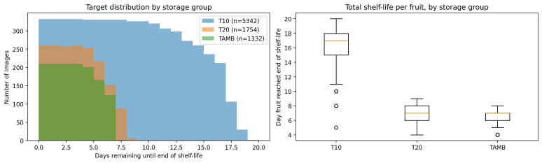
Refrigerated fruit survived 2.4 times longer than fruit at 20 °C (Table 2, Figure 1), confirming that the storage treatment produced a large and measurable difference in ripening rate — the premise on which the study rests. T20 and Tamb produced closely similar shelf-lives (6.77 and 6.34 days), consistent with ambient laboratory temperature having been near 20 °C.

Data Splitting

Each avocado contributes roughly twenty photographs across its observation period. Splitting at the image level would place photographs of the same physical fruit into both training and test partitions, allowing a model to score well by recognising individual fruit rather than by learning ripeness. All splits were therefore performed at the level of fruit identity.

Rather than a single fixed partition, we used repeated grouped cross-validation so that every fruit is tested exactly once per repeat and the estimate does not depend on one arbitrary split. The 401 retained fruit were divided into five folds stratified by storage group; within each fold assignment one fold served as the test set, the next as validation, and the remaining three as training, giving a 60 / 20 / 20 division. This was repeated twice with different fold assignments, yielding ten train/validation/test configurations. A programmatic assertion verified after every split that no fruit identifier appeared in more than one partition, and that the fold assignments were computed once and shared identically across every model configuration, so that configurations differ only in their input and never in which fruit they are tested on. We also confirmed that the distribution of shelf-life within each storage group was balanced across the training, validation and test partitions of every fold, so that no partition was enriched for faster- or slower-ripening fruit; per-group, per-partition shelf-life summaries are reported in the supplementary material. The validation partition drove early stopping, learning-rate scheduling and best-checkpoint selection; the test partition was evaluated once per fold.

Because the fold assignments were fixed before any group filtering, configurations restricted to a subset of storage groups (below) see exactly the corresponding subset of the shared partitions rather than a fresh split.

Pre-processing and Augmentation

Source images were resampled once to 384 × 384 pixels using Lanczos filtering and re-encoded at JPEG quality 95, then cached to local storage. This was an input-pipeline optimisation rather than a modelling decision: both training and evaluation transforms reduce images to 224 × 224 regardless, so caching at 384 px performs most of that reduction once instead of repeating it every epoch. Measured mean pixel difference at 224 px between the cached and original pipelines was 0.83% (PSNR 39.2 dB).

Training images were augmented, each transform applied with probability 0.5 except the crop, which was always applied: random resized cropping to 224 × 224 (scale 0.85–1.0, bilinear interpolation), random horizontal and vertical flips, random rotation up to 20°, and random brightness, contrast and saturation jitter (each ± 0.15, saturation ± 0.10)¹⁹. Hue jitter was deliberately excluded, since colour is the primary visual ripeness signal and perturbing it would corrupt the label relationship¹⁹. Normalisation with ImageNet channel statistics² was applied after augmentation. Validation and test images were resized so that the shorter side was 255 pixels (bilinear) and centre-cropped to 224 × 224, with no augmentation. All resampling used bilinear interpolation.

Environmental Encoding

T10 and T20 conditions are documented precisely (10 °C and 20 °C, both at 85% relative humidity). Ambient conditions are not. The originating study reports that the room-temperature group experienced “natural daily oscillations in temperature that ranged between 15.8 °C and 21.7 °C, with an average of 18.7 °C and a standard deviation of 1.2 °C,” and states explicitly that “due to technical difficulties, it was not possible to track the RH of this environment”¹⁸.

Ambient temperature is therefore set to the reported mean of 18.7 °C rather than assumed, and its sensitivity to misspecification is tested by sweeping the value across the full reported 15.8–21.7 °C range. No humidity value is imputed for the ambient group. Configurations that use relative humidity are restricted to T10 and T20, where it was actually recorded; the encoder raises an error rather than substituting a value if humidity is requested for a group lacking it.

Because temperature, humidity and storage-group identity are mutually collinear across only three treatment groups, the environmental input is not supplied as a single fixed vector. Channels are selected per configuration so their contributions can be separated (Table 5).

Model Architecture

All configurations share a common late-fusion design so that they differ in input only, not in architectural family:

• Image branch: ResNet-18⁴, ImageNet-pretrained², fully fine-tuned, final classification layer replaced by an identity mapping to yield a 512-dimensional embedding. This branch is present and identical in every configuration.
• Environment branch: a two-layer multilayer perceptron with ReLU activations, taking whichever environmental channels the configuration supplies. Its input width varies with the configuration; its hidden width (32) does not.
• Fusion head: concatenated features passed through dropout (p = 0.2), a 128-unit fully connected layer with ReLU, further dropout, and a single linear output producing a scalar prediction in days.

The submitted version of this work compared only three configurations and, in doing so, supplied the environment as a single five-element vector combining standardised temperature, standardised humidity and a three-element storage-group one-hot. With only three storage groups these channels are mutually collinear — the one-hot alone already identifies the treatment — so removing the whole vector at once cannot reveal which channel carries any gain. To separate them, eight configurations were evaluated on identical fruit folds with an identical image branch (Table 3):

Configuration	Environmental input	Question addressed
image_only	none	Can appearance alone predict days remaining?
image_zero_env	all channels, values zeroed	Does the environment MLP’s extra capacity alone help?
image_shuf_env	all channels, permuted across fruit	Does the branch help without valid information?
image_temp	continuous temperature	Does temperature add to vision?
image_group1hot	storage-group one-hot	Does categorical storage identity add to vision?
image_rh	relative humidity (T10, T20)	Does humidity add to vision?
image_temp_rh	temperature + humidity (T10, T20)	Do the recorded physical variables together add?
image_env_full	temperature + storage-group one-hot	Does the fullest defensible environment help?

Two of these are controls rather than models of interest. image_zero_env carries the same environmental branch and parameter count as the full model but with every environmental value set to zero; image_shuf_env carries valid environmental values permuted across fruit, so the branch receives information of the right type but wrong for each fruit. Any improvement these controls show over image_only is attributable to the added parameters, not to environmental information — the distinction the submitted version could not make. The image_rh and image_temp_rh configurations are restricted to the T10 and T20 groups, the only groups for which humidity was recorded.

Training

Models were implemented in PyTorch²⁰ and trained with the AdamW optimiser²¹ (learning rate 2 × 10⁻⁴, weight decay 1 × 10⁻⁴), batch size 64, for a maximum of 30 epochs with early stopping on validation MAE (patience 6) and learning-rate reduction on plateau. Huber loss (δ = 2.0) was used rather than squared error, for robustness to the long tail of very-underripe fruit. Mixed-precision training was enabled. Weights from the best validation epoch were retained for test evaluation. The learning rate and the Huber δ follow standard practice for this architecture and were fixed in advance rather than tuned on the evaluation folds; because every reported comparison is between configurations trained under these identical settings, the attribution result is robust to their exact values — a change would shift all configurations together.

Each of the eight configurations was trained on all ten cross-validation folds at a fixed random seed, for eighty training runs in total. Random seeds address a different source of variability from the cross-validation folds: the folds measure how the result varies across fruit, whereas the seed measures how it varies across training runs of the same data. To confirm that training was stable across initialisations, the two reference configurations — image_only and image_env_full — were additionally trained under two further seeds (123, 456).

Evaluation Metrics

Fruit-weighted error. The submitted version reported MAE over images, which over-weights long-lived fruit because they contribute more daily photographs — the refrigerated group alone supplies 63% of the retained images. Because the biologically independent unit is the fruit, not the photograph, the primary metric is a fruit-weighted MAE: mean absolute error is computed per fruit and then averaged across fruit, so every avocado counts equally regardless of how many times it was photographed. Image-weighted MAE is also reported for comparability with prior work.

Confidence intervals by bootstrapping fruit. For each configuration we report the paired improvement over the image-only baseline — the per-fruit difference in MAE — with a 95% confidence interval obtained by bootstrapping over fruit (10,000 resamples), not over photographs. Resampling photographs would treat the roughly twenty images of one avocado as twenty independent observations and produce a spuriously narrow interval. An interval that excludes zero indicates the configuration improves on image-only beyond fruit-to-fruit variability.

Per group. Fruit-weighted MAE computed separately for each storage group.

Normalised MAE (nMAE). Per-group MAE divided by that group’s mean shelf-life. Because T10 fruit live approximately 2.4 times longer than T20 fruit, raw MAE is not comparable across groups; nMAE expresses error as a fraction of the fruit’s total lifespan.

Baselines

Two non-learned baselines were fitted on each training fold and evaluated on the held-out fold, on identical footing with the models:

1. Constant — predict the training-fold median days-remaining for every image.
2. Group median — predict each storage group’s training-fold median. This is the value obtainable from storage condition alone, with no image, and is the value image-only must beat to show that appearance contributes beyond knowledge of storage condition.

Experiment 2: Can Appearance Reveal Storage Temperature?

To interpret the ablation, we trained a separate ResNet-18 classifier to predict storage group from images alone. High accuracy would indicate that visual features already encode thermal history, rendering an explicit temperature channel largely redundant; low accuracy would indicate the channel supplies genuinely new information.

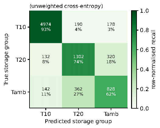
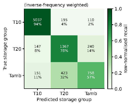
Because the retained dataset is imbalanced (63.4% T10), this experiment was run twice: once with standard cross-entropy, and once with inverse-frequency class weighting, , to separate genuine visual ambiguity from majority-class bias.

Sensitivity Analysis

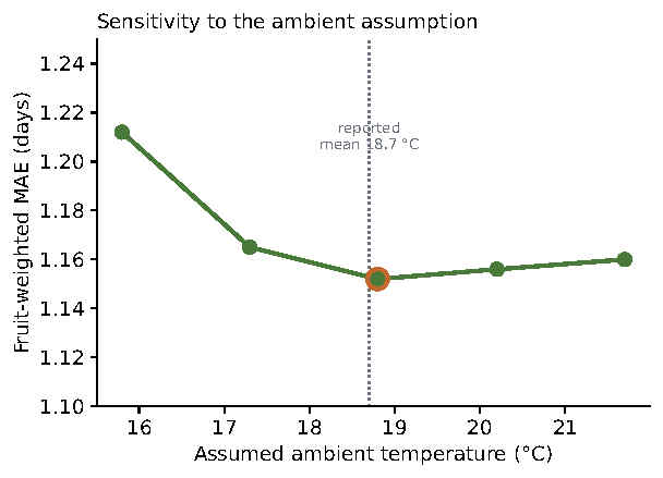
The ambient group’s temperature enters the model as a single assumed value (18.7 °C) standing in for a quantity that actually fluctuated between 15.8 and 21.7 °C. To test how much this assumption affects the result, the temperature configuration was re-trained five times with the ambient value set to each of five points spanning that full range, everything else held fixed. If the prediction were sensitive to the assumption, error would change materially across the sweep.

Hardware and Reproducibility

All experiments were conducted on an NVIDIA T4 GPU using PyTorch²⁰. The eight-configuration ablation across ten folds, the ambient-temperature sweep, and the storage-condition classifier together required roughly seventy GPU-hours. Random seeds were fixed for splitting and training. Every prediction was written to a single canonical file from which all tables and figures are derived, so that no reported count can disagree with another; that file, the derived tables, per-run training histories and model checkpoints were retained.

Results

Baselines

Predictor	Inputs	Fruit-weighted MAE (d)
Constant (overall median)	none	3.309
Group median	storage condition only	2.711
image-only (Table 5)	image only	1.658
image + storage condition (Table 5)	image + storage condition	1.126

The four rows of Table 4 establish the paper’s premise directly. Knowing only the storage condition, with no image at all, already improves on a constant predictor (2.711 vs 3.309 days), so storage condition carries genuine signal on its own. But appearance carries more: the image-only model (1.658 days) comfortably beats the storage-only baseline. Neither is sufficient alone — combining them reaches 1.126 days, better than either. Appearance and storage condition are complementary sources of information, which is precisely why supplying both matters.

Main Ablation

Configuration	Environmental input	Fruit-weighted MAE (d)	Δ vs image-only (d)	95% CI
image_only	none	1.658	—	—
image_zero_env	zeroed (capacity control)	1.652	0.007	[−0.031, 0.044]
image_shuf_env	permuted (information control)	1.620	0.039	[−0.002, 0.078]
image_group1hot	storage-group one-hot	1.137	0.521	[0.450, 0.593]
image_temp	continuous temperature	1.130	0.529	[0.458, 0.600]
image_env_full	temperature + one-hot	1.126	0.533	[0.462, 0.605]

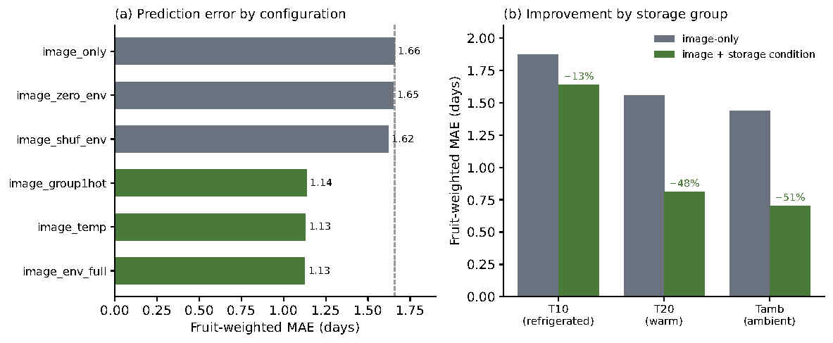
Supplying storage condition reduced fruit-weighted MAE from 1.658 to 1.126 days, a 32% improvement, with a confidence interval [0.462, 0.605] days that comfortably excludes zero (Table 5, Figure 2a). Three findings follow, each addressing a specific concern about the submitted version.

The gain is information, not capacity. The two controls carry the environment branch and its full parameter count but no usable signal. Neither improves on image-only to significance: zeroing the environmental values leaves MAE essentially unchanged (Δ 0.007, CI [−0.031, 0.044]), and permuting valid values across fruit is almost as inert (Δ 0.039, CI [−0.002, 0.078]). Because these architecturally larger models do not beat the pure image model, the improvement from the real configurations reflects the environmental information they receive, not the extra parameters — a distinction the submitted version, which removed the whole environmental vector at once, could not establish.

The gain is not attributable to temperature specifically. Continuous temperature (Δ 0.529) and the categorical storage-group one-hot (Δ 0.521) produce statistically indistinguishable improvements, their confidence intervals almost entirely overlapping. Supplying both together (image_env_full, Δ 0.533) is no better than either alone. With only three storage regimes the one-hot already identifies the treatment, and the continuous temperature value carries no additional predictive information. The improvement is therefore correctly attributed to knowledge of storage condition, not to temperature as a continuous physical variable — the correction this revision makes to the submitted title and claims.

Humidity contributes nothing, and slightly hurts. On the T10 + T20 subset where humidity was recorded, adding it alone made predictions worse than image-only (image_rh, Δ −0.083, CI [−0.139, −0.028]), while temperature-plus-humidity (image_temp_rh, Δ 0.422 on the same subset) did not exceed temperature alone. This is expected: recorded relative humidity was a constant 85% for both T10 and T20, so it carries no information distinguishing them and merely adds a noisy input dimension.

Per-Group Contribution

Group	Mean shelf-life (d)	image-only	image_env_full	Δ (d)	95% CI	Improvement
T10	16.10	1.876	1.640	0.236	[0.157, 0.316]	12.6%
T20	6.77	1.559	0.810	0.749	[0.623, 0.876]	48.0%
Tamb	6.34	1.436	0.702	0.734	[0.569, 0.909]	51.1%

The contribution of storage condition is significant in every group — all three confidence intervals exclude zero — but strongly non-uniform (Figure 2b). It is smallest for refrigerated fruit (0.236 days, 12.6%) and roughly three times larger for the two room-temperature groups (0.749 and 0.734 days, 48–51%). Refrigerated fruit ripen slowly and are visually distinctive, so appearance alone already predicts them reasonably well and storage context adds least; the short-lived room-temperature fruit, whose entire remaining lifespan is around six days, are where knowing the storage condition matters most.

The temperature-versus-category equivalence seen overall also holds within each group, and the way it holds is telling. In the refrigerated group continuous temperature is marginally ahead of the one-hot (0.250 vs 0.214 days); in the ambient group the one-hot is marginally ahead (0.733 vs 0.693). Neither difference is significant, and the direction reverses between groups — exactly the pattern expected when two inputs carry the same information and differ only by sampling noise, and not what would be seen if the continuous temperature value held genuine extra signal.

Experiment 2: Storage Condition Inference from Images

The per-group gradient above raises a natural question: does appearance already reveal a fruit’s storage condition, and if so, how well? To answer it we trained a separate image-only classifier to predict storage group, pooling one cross-validation repeat so that every fruit is classified exactly once. All figures below derive from a single saved prediction file, so the confusion matrices, per-class recalls and accuracies are mutually consistent by construction.

Group	Support (images)	Recall (unweighted)	Recall (weighted CE)
T10	5,342	0.931	0.943
T20	1,754	0.742	0.779
Tamb	1,332	0.622	0.569

Overall accuracy was 0.843 against a majority-class baseline of 0.634 (Table 7), and inverse-frequency class weighting changed it negligibly (0.850; macro recall 0.765 → 0.764; Figure 4). The confusion matrices show that weighting merely redistributes a little recall between the room-temperature groups without adding information — the same conclusion the submitted version reached, now on consistent counts.

The structure of the errors is the informative part. Refrigerated fruit are the most visually distinctive (recall 0.931), and the cold-versus-warm distinction is strong: pooled across the two room-temperature groups, 91.1% of warm fruit are correctly identified as warm rather than cold. What the classifier struggles with is the within-warm distinction — T20 and Tamb are confused with each other far more than either is confused with T10 — which is unsurprising, since 10 °C refrigeration produces a visibly slower, greener fruit while 18.7 °C and 20 °C produce very similar appearances.

Group	Image recall (visual identifiability)	Storage-condition benefit (Table 6)
T10 (refrigerated)	0.931	12.6%
T20	0.742	48.0%
Tamb	0.622	51.1%

The two experiments line up in rank order (Table 8): the more identifiable a storage condition is from appearance alone, the less the regressor gains from being told it. Refrigerated fruit are the most visually distinctive and gain the least (12.6%); ambient fruit are the least distinctive and gain the most (51.1%). The relationship is looser than the submitted version claimed — the room-temperature groups are partly identifiable, not near-random — but the qualitative correspondence holds and now rests on internally consistent counts. It also has a second component beyond visual ambiguity: the room-temperature groups are short-lived (≈ 6 days), so any error the regressor makes in inferring the ripening rate consumes a large fraction of the remaining lifespan, whereas the same relative error is diluted across the refrigerated group’s ≈ 16-day span.

Sensitivity to the Assumed Ambient Temperature

The ambient group’s temperature was not recorded continuously but summarised as a mean of 18.7 °C over a range of 15.8–21.7 °C. Because that single value feeds the environmental branch, its misspecification is a legitimate concern. We therefore re-ran the temperature configuration five times, holding everything else fixed and setting the ambient temperature to each of five values spanning the full reported range.

Assumed ambient temperature (°C)	Fruit-weighted MAE (d)
15.8 (cold extreme)	1.212
17.3	1.165
18.8 (≈ reported mean)	1.152
20.2	1.156
21.7 (warm extreme)	1.160

The result is insensitive to the assumption (Table 9, Figure 5). Across the entire 15.8–21.7 °C range the fruit-weighted MAE varies by only 0.06 days, and the minimum falls at 18.8 °C — essentially the dataset’s reported 18.7 °C mean. Even the worst choice, the cold extreme, raises error by about 5% relative to the optimum. Misspecifying the ambient temperature anywhere within its real range therefore has a negligible effect on prediction.

This concern is in any case doubly mitigated. The main ablation showed that the improvement is carried equally by the categorical storage-group indicator, which does not use the temperature value at all; so the configuration a deployed model would rely on is entirely invariant to the ambient assumption, and even the temperature-based configuration proves robust to it.

Discussion

Restatement of Key Findings

Supplying a CNN with a fruit’s storage condition alongside a photograph reduced days-remaining error by 32%, from a fruit-weighted 1.66 to 1.13 days, with a bootstrap confidence interval over fruit that excludes zero. Two controls establish that the gain is environmental information rather than added model capacity, and a further comparison shows that a categorical storage indicator does as well as a continuous temperature value — so across these three storage regimes the improvement is attributable to storage condition, not to temperature as a continuous physical variable. The improvement is not uniform: it ranges from 12.6% for refrigerated fruit to 51.1% for ambient-stored fruit.

A second experiment helps explain that gradient. An image-only classifier identifies refrigerated fruit most reliably (recall 0.93) and the two room-temperature conditions less well (0.62–0.74), and the rank order of visual identifiability matches the rank order of benefit inversely: the more clearly appearance reveals a storage condition, the less the regressor gains from being told it explicitly. Class-weight correction changes this negligibly, confirming the pattern reflects genuine visual signal rather than class imbalance.

Interpretation: State Versus Rate

We propose a straightforward mechanism. A photograph reveals a fruit’s current state; it does not reliably reveal the rate at which that state will change. Presented with a single image, a vision-only model cannot always distinguish a refrigerated fruit with ten days remaining from a room-temperature fruit with three, and must hedge between them. That hedge is costly precisely for the short-lived warm groups, whose entire remaining lifespan is around six days, so that an error in the inferred ripening rate consumes a large fraction of it. Supplying the storage condition collapses much of the ambiguity. The same logic has long been recognised in non-vision sensing: an ultrasonic measurement of avocado firmness indexes a fruit’s current state, but its mapping to remaining shelf-life shifts with the fruit’s prior time–temperature history²², and mechanistic kinetic models represent ripening with fitted initial conditions and Arrhenius temperature-dependent rate constants¹⁰.

An important qualification follows from the ablation. Because a three-level categorical indicator does as well as a continuous temperature value, the model is not learning the smooth, Arrhenius-type dependence of ripening rate on temperature that post-harvest physiology describes⁸. It is learning that three discrete storage regimes ripen at three different rates. Whether a vision model can recover the continuous law — rather than a lookup over a handful of conditions — cannot be settled with only three temperatures and is left to datasets that sample temperature more finely. The present claim is the narrower and better-supported one: knowing which of a small number of storage regimes a fruit is in substantially improves the prediction.

Connection to Prior Work

Our results extend the dataset’s originating study, which used the same 478 avocados for five-stage classification (88.8% accuracy) but did not attempt days-remaining regression or isolate the storage variable, despite having collected the necessary data¹⁸.

The result also sits alongside the shelf-life regression literature. Jada et al. reported MAE 1.44 days for banana using RGB images with day labels derived from stage class names under a fixed-rate assumption⁷; our image-plus-storage configuration reached a fruit-weighted 1.13 days with measured labels. Davur et al. reported 1.17 days for avocado using hyperspectral imaging of 80 fruit⁶, and Han et al. reported an RMSE of 1.43 days for ‘Hass’ using deep-network regression on single hyperspectral images of 316 ‘Hass’ fruit²³; our per-group errors of 0.810 days (T20) and 0.702 days (Tamb) are of comparable magnitude using ordinary RGB photography plus a storage-condition label. These comparisons must be read cautiously — the studies differ in fruit, dataset, imaging modality, split protocol and target definition, and our long-lived refrigerated group spans a much wider target range, which inflates its MAE mechanically. They indicate that RGB-plus-metadata is competitive with more elaborate sensing, not that it is superior.

More broadly, the finding is consistent with the multi-modal fusion literature, in which adding a non-visual modality to imaging improves produce assessment^14,24. Our contribution is not to add another such demonstration but to decompose one: by holding the image branch fixed and varying only the environmental input — including controls that add the branch’s parameters without its information — we separate the contribution of the environmental channel from the capacity it brings, and the contribution of a continuous temperature from that of a categorical storage label. That decomposition, rather than the existence of a fusion benefit, is what distinguishes this study.

Practical Implications

For anyone building a consumer-facing ripeness tool, the finding is directly actionable, and the specific form of the finding matters. A photograph-only application would forgo roughly a third of achievable accuracy overall, and about half for room-temperature fruit — which is how most consumers store avocados. But because a categorical storage label does as well as a continuous temperature, the input the application needs is not a precise measurement. It is simply which regime the fruit is in — refrigerated or left out — a single choice a user can supply directly, with no thermometer, weather lookup or sensor. This is both cheaper and more reliable than attempting to infer an indoor fruit’s temperature from external data, and the ablation shows nothing is lost by it.

The asymmetry has a practical corollary: storage information matters least for refrigerated fruit, which the model can already recognise from appearance, and most for counter-stored fruit, which is the common case.

Limitations

Right-censoring is uneven. 16.1% of fruit never reached stage 4 and were excluded, but the rate varied from 9.1% (T20) to 26.6% (Tamb). The retained Tamb sample is therefore biased toward faster ripeners, and its measured 6.34-day mean shelf-life is likely an underestimate. The apparent difference between T20 and Tamb should not be read as a physical effect. This does not threaten the main finding, which concerns the contribution of storage information rather than the absolute shelf-life of any group, and which holds within each group separately (Table 6), including the less-censored T20; but a dataset with complete observation would let the ambient group’s true distribution be estimated rather than bounded.

Ambient conditions are only partly documented. T10 and T20 are specified precisely; the ambient group is not. Its temperature was not held constant but oscillated between 15.8 °C and 21.7 °C, and its humidity was never recorded¹⁸. Ambient temperature therefore enters the model as a single summary value (18.7 °C) standing in for a fluctuating quantity, and the ambient group contributes no humidity information at all. The sensitivity sweep across the full reported temperature range quantifies how much this matters; the humidity gap is unrecoverable and is handled by excluding the ambient group from humidity-based configurations rather than by imputation.

Class imbalance. Refrigerated fruit constitute 63.4% of retained images, because longer-lived fruit yield more daily photographs. The submitted version’s image-weighted metrics let this inflate the refrigerated group’s influence; the present analysis reports fruit-weighted error as its primary metric, so every fruit counts equally regardless of how often it was photographed, and reports per-group results throughout. The imbalance remains in the training data itself, which the storage-condition classifier’s weighting experiment addresses directly.

Storage condition is a treatment label, not a continuous measurement. The model receives which of three regimes a fruit was kept in, not a logged temperature trace — and the ablation shows this is all the present data can support, since a categorical label already captures the available signal. Performance under continuously varying real-world temperature, and whether finer temperature sampling would let a model exploit a continuous rate law, remain untested.

Only three storage conditions. The central attribution result — that a categorical label does as well as a temperature value — is a direct consequence of having three regimes, among which temperature, humidity and identity are collinear. It correctly bounds what this dataset can show, but a study spanning many temperatures could in principle separate a continuous temperature effect from a categorical one, which this design cannot.

Single cultivar, single dataset, laboratory conditions. All images derive from one controlled study of Hass avocados against consistent backgrounds. Generalisation to other cultivars, other fruit species, and photographs taken in uncontrolled consumer settings is unverified.

Limited architectural exploration. ResNet-18 was used throughout, deliberately, to keep the eight-configuration comparison controlled; a single backbone means the absolute error, though not the relative contribution of storage condition, might differ with a deeper or more modern architecture.

No interpretability analysis. The model’s visual reasoning was not inspected. Gradient-weighted class activation mapping²⁵ would indicate whether predictions rest on physiologically meaningful features such as skin darkening.

Recommendations for Future Work

The most direct extension follows from the central limitation. A dataset spanning many storage temperatures, rather than three, would allow the decisive test this study could not perform: whether a vision model conditioned on temperature learns the smooth Arrhenius dependence of ripening rate⁸, or continues to behave as a lookup over discrete regimes. The natural endpoint is a model conditioned not on where a fruit is stored but on the cumulative thermal exposure it has actually accumulated. Beyond that, testing cross-cultivar and cross-dataset transfer would establish whether “ripeness” is a transferable visual concept²³; adding interpretability analysis such as gradient-weighted class activation mapping²⁵ would show whether predictions rest on physiologically meaningful features such as skin darkening; and validating on photographs captured by consumers rather than in a laboratory would be a prerequisite for deployment.

Two further directions bear on deployment specifically. A days-remaining estimate is only useful with a calibrated notion of its uncertainty, so that a stated range covers the true value at its claimed rate; conformalised quantile regression provides distribution-free prediction intervals with finite-sample coverage, and post-hoc recalibration offers an asymptotically calibrated alternative; both are natural complements to the fruit-level bootstrap intervals reported here^26,27. Separately, vision–language models offer a route to fine-grained produce assessment that generalises across fruit types with little labelled data, and adapting them to ripeness could reduce the per-cultivar data cost that a purely supervised model like ours incurs²⁸.

Closing Thought

Deep learning applied to fruit imagery has largely proceeded as though a photograph contains everything worth knowing. It does not. A photograph is a snapshot of state, and state alone cannot tell you how fast the future is arriving. Knowing where a fruit has been stored supplies what the image cannot, cutting the remaining error by roughly a third. What our data cannot yet show is whether a model can learn the continuous temperature dependence that post-harvest kinetics predicts: with only three storage regimes, a categorical label of the condition does just as well as its temperature. Testing whether finer temperature sampling lets a vision model recover that continuous law is the natural next step — but the broader lesson already holds, that appearance and storage context answer different questions and a useful predictor needs both.

References

1. A. Krizhevsky, I. Sutskever, G. E. Hinton. ImageNet classification with deep convolutional neural networks. Advances in Neural Information Processing Systems. Vol. 25, 2012. [↩]
2. J. Deng, W. Dong, R. Socher, L. J. Li, K. Li, L. Fei-Fei. ImageNet: a large-scale hierarchical image database. Proceedings of the IEEE Conference on Computer Vision and Pattern Recognition. pg. 248–255, 2009. [↩] [↩] [↩]
3. M. Rizzo, M. Marcuzzo, A. Zangari, A. Gasparetto, A. Albarelli. Fruit ripeness classification: a survey. Artificial Intelligence in Agriculture. Vol. 7, pg. 44–57, 2023, https://doi.org/10.1016/j.aiia.2023.02.004. [↩]
4. K. He, X. Zhang, S. Ren, J. Sun. Deep residual learning for image recognition. Proceedings of the IEEE Conference on Computer Vision and Pattern Recognition. pg. 770–778, 2016. [↩] [↩]
5. F. M. A. Mazen, A. A. Nashat. Ripeness classification of bananas using an artificial neural network. Arabian Journal for Science and Engineering. Vol. 44, pg. 6901–6910, 2019, https://doi.org/10.1007/s13369-018-03695-5. [↩]
6. Y. J. Davur, W. Kämper, K. Khoshelham, S. J. Trueman, S. Hosseini Bai. Estimating the ripeness of Hass avocado fruit using deep learning with hyperspectral imaging. Horticulturae. Vol. 9, pg. 599, 2023, https://doi.org/10.3390/horticulturae9050599. [↩] [↩]
7. S. S. C. Jada, M. Senthil, K. Vivek. Classification vs. regression for real-time fruit shelf-life prediction: a transfer learning approach with MobileNetV2 for edge AI. International Journal of Computer Applications. Vol. 187, pg. 50–57, 2025. [↩] [↩] [↩]
8. C. R. Chen, H. S. Ramaswamy. Color and texture change kinetics in ripening bananas. LWT — Food Science and Technology. Vol. 35, pg. 415–419, 2002, https://doi.org/10.1006/fstl.2001.0875. [↩] [↩] [↩]
9. I. L. Eaks. Ripening, respiration, and ethylene production of ‘Hass’ avocado fruits at 20° to 40 °C. Journal of the American Society for Horticultural Science. Vol. 103, pg. 576–578, 1978, https://doi.org/10.21273/jashs.103.5.576. [↩]
10. S. G. Gwanpua, Z. Qian, A. R. East. Modelling ethylene regulated changes in ‘Hass’ avocado quality. Postharvest Biology and Technology. Vol. 136, pg. 12–22, 2018, https://doi.org/10.1016/j.postharvbio.2017.10.002. [↩] [↩]
11. N. M. Sierra, A. Londoño, J. M. Gómez, A. O. Herrera, D. A. Castellanos. Evaluation and modeling of changes in shelf life, firmness and color of ‘Hass’ avocado depending on storage temperature. Food Science and Technology International. Vol. 25, pg. 370–384, 2019, https://doi.org/10.1177/1082013219826825. [↩]
12. A. Ogawa, M. Terakado, R. Nakadate, R. Chiba, N. Yamamoto. A practical approach for predicting avocado ripeness using a portable Vis-NIR device and sensory-based indexing under various storage temperatures. AgriEngineering. Vol. 8, pg. 130, 2026, https://doi.org/10.3390/agriengineering8040130. [↩]
13. R. Singh, R. Nisha, R. Naik, K. Upendar, C. Nickhil, S. C. Deka. Sensor fusion techniques in deep learning for multimodal fruit and vegetable quality assessment: a comprehensive review. Journal of Food Measurement and Characterization. Vol. 18, pg. 8088–8109, 2024, https://doi.org/10.1007/s11694-024-02789-z. [↩]
14. Y. Liu, C. Wei, S.-C. Yoon, X. Ni, W. Wang, Y. Liu, D. Wang, X. Wang, X. Guo. Development of multimodal fusion technology for tomato maturity assessment. Sensors. Vol. 24, pg. 2467, 2024, https://doi.org/10.3390/s24082467. [↩] [↩]
15. K. Yang, S. Jung, J. Lee, U. Jung, M. Lee. Prediction of optimal harvest timing for melons through integration of RGB images and greenhouse environmental data: a practical approach including marker effect analysis. Agriculture. Vol. 16, pg. 169, 2026, https://doi.org/10.3390/agriculture16020169. [↩]
16. B. H. Cho, S. Koseki. Determination of banana quality indices during the ripening process at different temperatures using smartphone images and an artificial neural network. Scientia Horticulturae. Vol. 288, pg. 110382, 2021, https://doi.org/10.1016/j.scienta.2021.110382. [↩]
17. P. Xavier, P. Rodrigues, C. L. M. Silva. ‘Hass’ avocado ripening photographic dataset. Mendeley Data. 2024, https://doi.org/10.17632/3xd9n945v8.1. [↩] [↩]
18. P. Xavier, P. M. Rodrigues, C. L. M. Silva. Shelf-life management and ripening assessment of ‘Hass’ avocado (Persea americana) using deep learning approaches. Foods. Vol. 13, pg. 1150, 2024, https://doi.org/10.3390/foods13081150. [↩] [↩] [↩] [↩]
19. C. Shorten, T. M. Khoshgoftaar. A survey on image data augmentation for deep learning. Journal of Big Data. Vol. 6, pg. 60, 2019, https://doi.org/10.1186/s40537-019-0197-0. [↩] [↩]
20. A. Paszke, S. Gross, F. Massa, A. Lerer, J. Bradbury, G. Chanan, T. Killeen, Z. Lin, N. Gimelshein, L. Antiga, et al. PyTorch: an imperative style, high-performance deep learning library. Advances in Neural Information Processing Systems. Vol. 32, 2019. [↩] [↩]
21. I. Loshchilov, F. Hutter. Decoupled weight decay regularization. International Conference on Learning Representations. 2019. [↩]
22. U. Flitsanov, A. Mizrach, A. Liberzon, M. Akerman, G. Zauberman. Measurement of avocado softening at various temperatures using ultrasound. Postharvest Biology and Technology. Vol. 20, pg. 279–286, 2000, https://doi.org/10.1016/S0925-5214(00)00138-1. [↩]
23. Y. Han, S. H. Bai, S. J. Trueman, K. Khoshelham, W. Kämper. Predicting the ripening time of ‘Hass’ and ‘Shepard’ avocado fruit by hyperspectral imaging. Precision Agriculture. Vol. 24, pg. 1889–1905, 2023, https://doi.org/10.1007/s11119-023-10022-y. [↩] [↩]
24. Y. Li, R. Qiu, S. Hou, M. Zhang, X. Wang. MMFNet-K: a multimodal data fusion network for nondestructive freshness assessment of multiple kiwifruit cultivars. Food Research International. Vol. 241, pg. 119749, 2026, https://doi.org/10.1016/j.foodres.2026.119749. [↩]
25. R. R. Selvaraju, M. Cogswell, A. Das, R. Vedantam, D. Parikh, D. Batra. Grad-CAM: visual explanations from deep networks via gradient-based localization. Proceedings of the IEEE International Conference on Computer Vision. pg. 618–626, 2017. [↩] [↩]
26. Y. Romano, E. Patterson, E. J. Candès. Conformalized quantile regression. Advances in Neural Information Processing Systems. Vol. 32, pg. 3543–3553, 2019. [↩]
27. V. Kuleshov, N. Fenner, S. Ermon. Accurate uncertainties for deep learning using calibrated regression. Proceedings of the 35th International Conference on Machine Learning. pg. 2796–2804, 2018. [↩]
28. Y. Zhang, Y. Shao, C. Tang, Z. Liu, Z. Li, R. Zhai, et al. E-CLIP: an enhanced CLIP-based visual language model for fruit detection and recognition. Agriculture. Vol. 15, pg. 1173, 2025, https://doi.org/10.3390/agriculture15111173. [↩]