Demystifying Friction in Rolling Motion: Static, Kinetic, and the Nature of Rolling Resistance

July 29, 2026

Abstract

The analysis of friction in rolling motion is a common source of confusion in introductory physics. Students often struggle to reconcile the existence of static friction with a moving object and are further confounded by the introduction of “rolling friction” as a distinct force. This paper clarifies the roles of static and kinetic friction for rigid bodies in rolling motion. Through a detailed analysis of examples—a rolling cart and a sphere in air and vacuum—we demonstrate that the force traditionally labeled as “rolling friction” in some textbooks is, in fact, static friction. We argue that for an ideal rigid body on a rigid surface, a separate rolling friction force does not exist. Instead, what is commonly termed “rolling friction” or “rolling resistance” should be understood as a collection of mechanical energy dissipation mechanisms that arise from the deformation of non-rigid bodies.

Introduction

Friction is a fundamental contact force, crucial for understanding motion in the everyday world. Introductory physics textbooks typically introduce static friction (f_s) and kinetic friction (f_k), distinguishing them by the presence or absence of relative motion between the surfaces in contact¹^,². Students generally grasp that a stationary object experiences static friction, while a sliding object experiences kinetic friction.

However, this distinction blurs for round, rolling objects. There have been physics education research papers on the origin of students’ misconception about tolling motions³^,⁴^,⁵, as well as, a plethora of papers⁶^,⁷^,⁸^,⁹ exploring various ways of effectively teaching students the concept of rolling motions. A rolling wheel, for instance, has a clear center-of-mass velocity (v_cm), leading students to question how static friction can possibly act upon it. Similarly, students may also believe that static friction alone can prevent a rigid, round object from rolling down an incline⁸, and that the magnitude of the force of static friction is always μ_sN (μ_s is the coefficient of static friction, N is the magnitude of the normal force)¹⁰^,¹¹. These are important misconceptions of static friction that would benefit from being addressed. This confusion is compounded when textbooks introduce “rolling friction“ as a third type of frictional force²^,¹². Suddenly, students are left wondering which friction force acts, and they may begin to label any friction on a rolling object as “rolling friction,” obscuring the true physics at play. For example, one study notes that a misconception regarding the equivalence of kinetic and rolling friction exists, and that ’rolling friction is used for rolling objects’¹⁰. Furthermore, students appear to have trouble distinguishing the situations where rolling resistance arises; one study determined that prior to teacher sequence designed to reduce misconceptions about rolling friction, the majority of students believed that a rigid sphere rolling on a rigid and rough surface would be slowed due to friction¹¹. Generally, students appear to have misconceptions about the role of friction in rolling motion³^,¹³, and about free-body diagrams describing such situations¹⁴. Although significant work has been done to address students’ misconceptions of static and kinetic friction¹⁵, not as much work exists that addresses confusion around rolling friction.

This article aims to resolve these ambiguities and provide a helpful clarification for understanding rolling motion that could complement preexisting methods, such as the learning sequence described in a previously mentioned study¹¹. We will dissect the dynamics of rolling motion to enhance clarity on the frictional forces involved. Our central thesis is twofold: (1) for a perfectly rigid body rolling on a rigid surface, the friction forces acting on it are static or kinetic; and (2) what is commonly referred to as “rolling friction“ is not a fundamental force itself, but rather a macro-scale term for the energy losses, or rolling resistance, which occurs when real, deformable bodies interact. We distinguish between rolling friction and rolling resistance. Although the mechanics discussed here are well established, introductory presentations often only briefly mention rolling friction and discuss it in a way that can obscure the distinction between the mechanisms of static and kinetic friction and the mechanism of rolling resistance. This paper develops an instructional framework to clarify those distinctions while remaining consistent with established classical mechanics, suitable for college students and advanced secondary students who have already been introduced to Newtonian mechanics.

We will proceed by first reviewing the characteristics of static and kinetic friction in the context of rolling. We will then critically examine the textbook definition of rolling friction. Through the analysis of concrete examples—a shopping cart and a sphere in both air and vacuum—we will demonstrate that the retarding force in these systems is best understood as static friction. Finally, we will re-frame rolling resistance as a manifestation of mechanical energy dissipation in non-rigid systems and discuss its primary physical causes.

Modeling Assumptions

To ensure reproducibility, the assumptions used throughout this work are explicitly stated here. Rigid bodies are not deformable unless otherwise stated. Surfaces are rigid and stationary unless otherwise stated. Rolling without slipping implies that the no-slip condition ( $v_{\mathrm{cm}} = R\omega$ ) is satisfied at all times. Static friction adjusts instantaneously up to a maximum magnitude of $\mu_s N$ . Kinetic friction has constant magnitude $\mu_k N$ and opposes relative motion. Air resistance is modeled using linear (low-speed) or quadratic (high-speed) drag laws depending on Reynolds regime¹². Bearing and axle losses are ignored in derivations. Energy losses in deformable bodies are not represented as contact forces in free-body diagrams. This is why we refer to it as rolling resistance instead of rolling friction.

Friction Forces in Rolling Dynamics

To build a foundation for our analysis, we must first precisely define the roles of static and kinetic friction for a rolling object. For the following discussion, we consider a rigid, circular object (e.g., a wheel or sphere) of radius R on a rigid, stationary surface. Its motion is characterized by its center-of-mass velocity, v_cm, and its angular velocity,ω.

Static Friction in Rolling Without Slipping

Static friction acts when the point of the object in contact with the surface is instantaneously at rest relative to that surface. For a rolling object, this condition is met when it rolls without slipping, a state defined by $v_{\mathrm{cm}} = R\omega$ . In this scenario, the point of contact is momentarily stationary. Static friction arises not from motion, but from a tendency to slip.

This tendency is created by acceleration. An external force or torque applied to the object will try to upset the $v_{\mathrm{cm}} = R\omega$ condition. The role of static friction is to oppose this tendency, enforcing the no-slip condition. Its direction is determined by the nature of this tendency. Let us consider three cases:

Acceleration: Consider a car’s driving wheel accelerating forward. The engine applies a torque that tries to make the wheel spin faster, creating a tendency for the bottom of the tire to slip backward relative to the ground (Rω has a tendency to be greater than v_cm). Static friction opposes this by acting forward on the tire, propelling the car.

Deceleration: When a car brakes, the brakes apply a torque that slows the wheel’s rotation. This creates a tendency for the bottom of the tire to slip forward (v_cm has a tendency to be greater than Rω). Static friction then acts backward on the tire, slowing the car down.

Constant Velocity: If a perfectly rigid object rolls on a perfectly rigid, rough, and level surface at constant velocity where v_cm=Rω , both the acceleration a_cm and angular acceleration α are zero. Applying Newton’s second law:

(1) $\begin{equation*}\sum F_x = ma_x = 0 \qquad \end{equation*}$

(2) $\begin{equation*}\sum \tau = I\alpha = 0 \qquad\end{equation*}$

Here $\sum \mathbf{F}$ and $\sum \tau$ are net force and net torque, respectively, on the rolling object. Since there are no external horizontal forces or torques acting on the object in addition to (potentially) friction, the force of static friction must be zero. It is also crucial to note that static friction does no work, as the point of application (the contact point) is not displaced while the force is acting.

The magnitude of static friction, $|f_s|$ , varies dynamically in order to maintain the no-slip condition. However, it is constrained by the relation $|f_s| \le \mu_s N$ , where $\mu_s$ is the coefficient of static friction and $N$ is the normal force. If the magnitude of the static friction force required to maintain the no-slip condition exceeds $\mu_s N$ , the no-slip condition can no longer be maintained, and the object begins to slip. Since the object is now slipping, there is relative motion between the object and the surface, and the friction force acting on it is no longer static friction; instead, the force has transitioned to kinetic friction. This transition can be observed with rapid acceleration and hard braking.

Kinetic Friction in Rolling with Slipping

Kinetic friction comes into play when the no-slip condition is violated, and the object slides as it rolls: $v_{cm} \neq R\omega$ . This includes scenarios like a skidding car or a spinning tire on ice.

The kinetic friction force always opposes the relative motion of the two surfaces in contact. Its direction is therefore determined by which side of the $v_{\mathrm{cm}} = R\omega$ equation is larger. Let us consider two cases:

If $v_{cm} > R\omega$ (e.g., a locked brake), the bottom of the object slides forward relative to the ground. Kinetic friction acts backward, opposing v_cm.

If $v_{cm} < R\omega$ (e.g., a spinning tire on ice), the bottom of the object slides backward. Kinetic friction acts forward, in the direction of v_cm.

Kinetic friction always dissipates mechanical energy, converting it to heat. However, it can simultaneously increase either the translational kinetic energy (in the second case above) or the rotational kinetic energy (in the first case) as the system evolves toward the no-slip condition, $v_{\mathrm{cm}} = R\omega$ . For another detailed and clear example on the role of kinetic friction in nudging the system towards the satisfaction of the no-slip condition, see the paper by Hierrezuelo & Carnero¹³. Their example gives a more concrete and quantitative treatment.

The Textbook Definition of “Rolling Friction”

Many popular introductory textbooks introduce the concept of rolling friction, often leading to the very misconceptions this paper addresses. For instance, Knight describes it as a constant retarding force, f_r=μ_rN, arising from the deformation of the rolling object or the surface¹². Young and Freedman similarly define it as the horizontal force needed to maintain constant speed, also assigning it a coefficient μ_r².

While these descriptions correctly identify that a real wheel requires a force to maintain constant speed, their presentation as a simple, constant force on a free-body diagram is problematic and increases confusion. It implies that “rolling friction” is a fundamental interaction, acting in a fashion similar to static and kinetic friction. The definitions are vague about its origin, its relationship to slipping, and whether it can be drawn as a distinct vector on a free-body diagram. Other texts, like Halliday, Resnick, and Walker¹, avoid the term altogether, which, while avoiding the misconception, leaves students without an explanation for why real everyday objects, such as a rolling ball, eventually come to a stop. This inconsistency is a potential cause for confusion for students.

Rigid Body Analysis: The “Rolling Friction” Force is Static Friction

The ambiguity surrounding rolling friction can be resolved by carefully analyzing the dynamics of rigid bodies. The classic textbook example used to introduce rolling friction — pushing a heavy cabinet on a cart versus sliding it directly on the floor — provides a useful illustrative case.

Deconstructing the Cart Example

The argument typically proceeds as follows: it is easier to move the cabinet on a cart because the “coefficient of rolling friction”,μ_r, is much smaller than the coefficient of kinetic friction, μ_k. However, this explanation is a macroscopic simplification that masks the true microscopic interactions.

A complete dynamical analysis requires separate free-body diagrams (FBD) for the cart body and its identical wheels, as shown in Figure 1. The cart body and the cabinet (mass M, excluding wheels) is pushed by a force F_P. It interacts with the wheels (total mass m) via a horizontal normal force F at the axle. The wheels interact with the ground via a total normal force N and a total horizontal frictional force f.

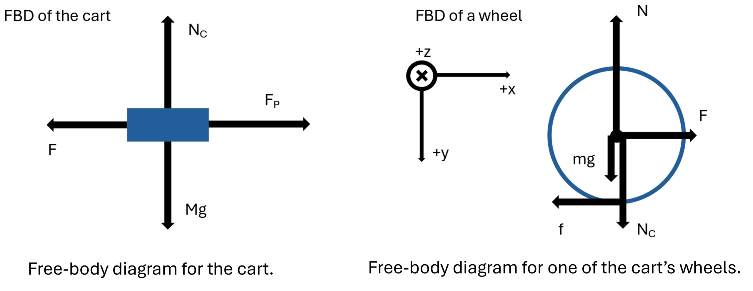
Figure 1 | Free-body diagrams for a cart and its wheels. The mass of the cart body and cabinet (excluding wheels) is M, and m is the total mass of all four wheels. F_P is the applied pushing force. N_C is the normal force between the cart and the wheels at the axle. F is the horizontal interaction force at the axle. N is the normal force from the ground. f is the frictional force from the ground.

Applying Newton’s laws to the cart yields:

(3) $\begin{equation*}\sum F_x = F_P - F = Ma_x\end{equation*}$

(4) $\begin{equation*}\sum F_y = Mg - N_c = 0 \end{equation*}$

For the collection of wheels, we have:

(5) $\begin{equation*}\sum F_x = F - f = ma_x\end{equation*}$

(6) $\begin{equation*}\sum F_y &= N_c + mg - N = 0\end{equation*}$

(7) $\begin{equation*} \sum \tau &= Rf = I\alpha\end{equation*}$

(8) $\begin{equation*}a_x &= R\alpha.\end{equation*}$

Equation 8 is the no-slipping condition, which is the hallmark of static friction. I is the total moment of inertia of all the wheels.

From these equations, we can see a clear causal chain. If the pushing force F_P increases, the acceleration $\alpha_x$ of the cart must increase (Eq. 3). To maintain the no-slip condition (Eq. 8), the angular acceleration of the wheels $\alpha$ must increase proportionally. This requires a larger torque, R_f, from the frictional force f (Eq. 7). Therefore, f must increase.

This analysis reveals the true nature of $f$ . It is not a constant, pre-determined “rolling friction” force ( $\mu_r N$ ). Instead, it is a variable force that adjusts in response to the applied push to satisfy the constraints of motion (rolling without slipping). This ability to vary between 0 and its maximum value, $\mu_s N$ , is one of the characteristics, but not the only characteristic, of static friction. The magnitude and direction of static friction adjust to enforce the no-slip condition ( $v_{cm}=R\omega$ ), up to a magnitude of $\mu_s N$ . Furthermore, since the contact points of the wheels with the ground are stationary with respect to the ground, the force $f$ is static friction, which acts to prevent the bottom of the wheel from slipping. In addition, the magnitude of $f$ depends on the acceleration of the cart, and not on a specific property of the rolling motion itself. The misconception of a separate, small “rolling friction” force arises from correctly observing that this static friction force is often very small.

Example: A Rolling Sphere in Air

The variable nature of this friction force is even more evident when we consider a rigid sphere rolling through air. Assume that a solid rigid sphere rolls without slipping on a level rigid surface and experiences air resistance. The air resistance magnitude on a moving object is proportional to the object’s center of mass speed: $D \propto v_{cm}^{\,n}$ , where $n=1$ for objects traveling at low speed (such as our rolling sphere example; more formally, the condition is that the Reynolds number is less than 1)¹²^,¹⁶^,¹⁷ and $n=2$ for traveling at higher speed (such as a driving car on a freeway, airplane, etc)¹²^,¹⁸. Similarly, the resistive torque due to the solid sphere rotating at low angular speed in air is proportional to its angular speed, i.e., $\tau_r \propto \omega$ , and $\tau_r \propto \omega^{2}$ at high angular speed¹⁹. Based on the above air drag and resistive torque discussions, we draw the FBD for a rigid solid sphere rolling without slipping on a rigid surface, as depicted in Figure 2.

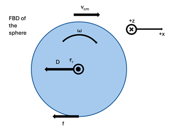
Figure 2 | Free-body diagram for a rigid sphere rolling without slipping on a horizontal surface in air. A drag force $D$ opposes translation, and a resistive torque $\tau_r$ (pointing out of the page) opposes rotation. A friction force $f$ is included at the contact point. Vertical forces are omitted for clarity.

The dynamical equations, assuming rolling without slipping ( $a_x = R\alpha$ ), are:

(9) $\begin{equation*}\sum F_x = -D-f = m a_x\end{equation*}$

(10) $\begin{equation*}\sum \tau = - \tau_r + Rf = I \alpha\end{equation*}$

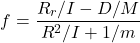
Solving for the friction force yields:

(11) $\begin{equation*}f = \frac{R \tu_r/I - D/M}{R^2 /I + 1/m}\end{equation*}$

Since our discussion is confined to the low speed regime (Stokes regime), the air drags are given by $\tau_r=8\pi\eta R^3\omega$ and $D=6\pi\eta Rv_{cm}$ , where $\eta=1.8\times10^{-5}\ \mathrm{Pa\cdot s}$ is the dynamic viscosity of air at $20^\circ\mathrm{C}$ ¹²^,¹⁶^,¹⁷^,¹⁹. It is worth noting that these two formulas assume an unbounded fluid and neglect wall-proximity corrections, which is known to be a higher order correction at low speed²⁰. The small correction will not change the qualitative argument presented in this paper. To obtain the value of friction force $f$ , we also make the following substitutions : I = (2/5)mR² for solid sphere. We end up with

$f = 4\pi \eta R \nu_{cm}$

A positive $f$ means the direction we assumed in the above FBD is correct²¹. A small dynamic viscosity value $\eta=1.8\times10^{-5}$ means that the friction force also has a tiny value. A rough estimate gives a friction force in the order of $10^{-5}\ \mathrm{N}$ for $R=0.11\ \mathrm{m}$ (soccer ball) and $v_{cm}=1\ \mathrm{m/s}$ . We also notice that the magnitude of the friction force $f$ depends on the center of mass velocity. Clearly, in our rolling sphere problem, $v_{cm}$ decreases over time, which means that the friction force decreases as well. This is strong evidence that the friction force in the rolling motion is definitely not a constant that can be described by the rolling friction formula: $f_r=\mu_r N$ , where $N$ is the normal force between the bottom of the sphere and the level surface. Instead, the friction force should be static friction, i.e., $f=f_s$ , which can take any value between $0$ and $\mu_s N$ , and can adjust its value during the sphere’s deceleration process to ensure that the no-slip condition holds.

Since static friction is closely tied to the concept of motion tendency of the contact surface between the sphere and the horizontal surface, we can also arrive at the same conclusion ( $f=f_s$ ) by exploring the motion tendency of the sphere. We first remove the friction force $f$ from Eq. 9 and Eq. 10, and solve for the linear and angular accelerations separately:

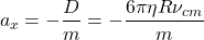
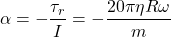
$\begin{equation*}a_x = -\frac{D}{m} = - \frac{6 \pi \eta R \nu_{cm}}{m}\end{equation*}$

$\begin{equation*}\alpha = - \frac{\tau_r}{I} = - \frac{20 \pi \eta R \omega}{m}\end{equation*}$

At the beginning, the solid sphere satisfies the no-slipping condition, i.e., $v_{cm}=R\omega$ . However, the angular speed $\omega$ would decrease at a higher rate than the center of mass speed $v_{cm}$ would, resulting in the bottom of the sphere’s tendency to slide forward, since $v_{cm}$ would be greater than $R\omega$ at the next instant if there were no friction force. The static friction, therefore, comes to the rescue and points backwards to oppose such a forward sliding tendency.

To conclude, only static friction was present in the example of rolling solid sphere in air. The above discussion is general, in the sense that it can be extended to any rolling object’s dynamics in air in the same way. However, the above discussion was intended as an illustrative low-Reynolds-number model rather than a mathematically formal discussion of a rolling sphere in contact with a surface. The drag and rotational resistance expressions also neglect boundary corrections associated with the nearby surface. Consequently, the above discussion is best interpreted as a qualitative demonstration that the required contact force remains static friction. It is possible that the misconception about the existence of a small rolling friction is caused by the tiny value of static friction in the rolling motion, which has tempted many authors to define a rolling friction force.

Example: A Rolling Sphere in a Vacuum

The most powerful argument against rolling friction as a fundamental force comes from considering an ideal system: a perfectly rigid sphere rolling on a perfectly rigid, level surface in a perfect vacuum. As shown in Figure 3, with no air resistance, D = 0 and τᵣ = 0.

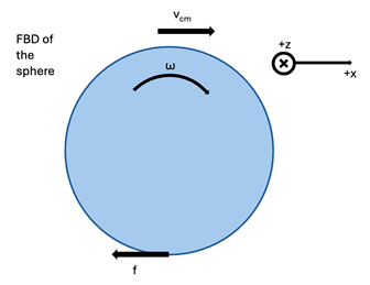Figure 3 | Free-body diagram for a rigid sphere rolling on a horizontal rigid surface in a vacuum. The only horizontal force considered is a hypothetical friction force $f$ , whose nature is under investigation.

If we attempt to include any horizontal friction force $f$ in our analysis, we encounter a logical contradiction. The equations of motion become:

(12) $\begin{equation*}\sum F_x = -f = ma_x\end{equation*}$

(13) $\begin{equation*}\sum \tau = Rf = I \alpha\end{equation*}$

A non-zero $f$ would simultaneously cause a deceleration in the linear direction ( $a_x<0$ ) and an acceleration in the rotational direction ( $\alpha>0$ ), violating the no-slipping condition that the sphere is presumably in. Since there are no external forces or torques, there is no mechanism to generates a tendency to slip. Therefore, the only physically consistent solution is that no friction force acts at all: $f=0$ . This can be further ascertained by plugging in $f=0$ into equations 12 and 13:

$\begin{equation*}\sum F_x = 0 = ma_x \Rightarrow a_x = 0\end{equation*}$

$\begin{equation*}\sum tau = 0 = I \alpha \Rightarrow \alpha = 0\end{equation*}$

Therefore,

$\omega(t) = \omega_0$

$\nu_{cm}(t) = \nu_0$

where the initial no-slip condition $v_{\mathrm{cm}} = R\omega$ still holds.

This thought experiment definitively shows that for a rigid body in the absence of other forces, the concept of a distinct “rolling friction” force is not only unnecessary but leads to a logical impossibility. The sphere would continue rolling at a constant speed forever, a testament to the fact that the only possible friction force for a rigid body is static friction, which is zero when no slipping tendency exists.

Rolling Resistance: Mechanical Energy Dissipation in Non-Rigid Bodies

If rigid bodies in a vacuum experience no frictional force, why do real-world objects like cars, bicycles, and balls eventually come to a stop? The answer lies not in a new type of force, but in the fact that real objects are not perfectly rigid. Their deformation during rolling leads to energy losses, a phenomenon best termed rolling resistance.

Real systems require a distinction between three levels of description: contact forces acting at the interface (static/kinetic friction), effective macroscopic models (e.g., rolling resistance forces used in engineering), and underlying dissipation mechanisms (hysteresis, deformation, micro-slipping) Rolling resistance is of the third kind; it should not be conceptualized as a contact force on a free-body diagram, but instead as a process of energy dissipation. Although its effect can be approximated by the macroscopic model of a constant “rolling friction force”, it is physically inaccurate; the true nature of rolling resistance is an underlying energy dissipation mechanism.

The primary mechanisms of this energy dissipation include hysteresis, shifted normal force, and micro-slipping. Each is discussed in more detail below.

Hysteresis & Shifted Normal Force

Hysteresis is the dominant cause of rolling resistance, accounting for the majority of the energy loss in a pneumatic tire²². It occurs in materials that are inelastic, such as rubber. As a non-rigid wheel rolls, the portion in contact with the ground is compressed. The material deforms to create a flat spot. As the wheel rotates, this section of the material must return to its original form as it leaves the contact patch. The work done to deform the material is not fully returned upon relaxation. In other words, the material behaves differently when being compressed and when returning to its original shape. As the energy is not fully returned with every rotation, it is instead converted into thermal energy. This is why the tires of a car heat up during a long drive; the energy lost to hysteresis manifests as thermal energy.

While hysteresis is an underlying dissipation mechanism, its effect on rolling motion can also be macroscopically described by a shifted normal force. Since both the surface and object are deformable, the contact area is not a single point. Furthermore, due to hysteresis, the object behaves differently when being compressed and when relaxing. This leads to a non-uniform pressure distribution across the contact patch. It is higher towards the leading edge of the contact patch and lower towards the trailing edge. The effect of this asymmetric pressure distribution is that the effective point of application of the normal force shifts slightly forward in the direction of motion²³. See Figure 4 for a visual representation; the offset normal force creates a torque $\tau=Nd$ about the center of the object that opposes the rotation and contributes to the deceleration. The effects of hysteresis on rolling motion can be represented using a shifted normal force, which can be estimated using the engineering approximation $f_r=\mu_r N$ .

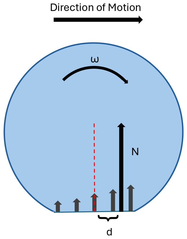Figure 4 | This is a diagram showing how the normal force acts at different positions across the contact patch. The gray arrows represent the normal force acting slices of the contact patch. As shown in the figure, the pressure distribution has its peak closer to the leading edge of the object (towards the direction of motion). The black arrow labeled $N$ represents the total normal force acting upon the object, and is obtained by summing all of the normal forces acting upon the slices of the contact patch. The dotted red line represents the horizontal center of the object. $d$ is the horizontal offset of the total normal force $N$ from the horizontal center of the object (red dotted line). The lengths of the normal force arrows are not to scale.

Partial-Slipping/Micro-Slipping

In the idealized rigid-body examples discussed earlier, the contact of the object with the ground was treated as only occurring at a single point. In reality, contact between two deformable bodies occurs over a contact patch. When a wheel rolls without slipping, the condition $v_{\mathrm{cm}} = R\omega$ applies to the wheel as a whole. However, the distribution of forces within the contact patch is more complex. As the wheel rolls, tangential stresses arise across the contact patch. These stresses are generally non-uniform. Due to these stresses, small portions of the contact patch may undergo localized slipping, while the remainder of the contact patch remains stuck to the surface. This phenomenon is known as partial-slipping, or micro-slipping. This slipping is not classified as kinetic friction, as only portions of the contact patch slide relative to the surface. Partial-slipping is confined to small localized regions of the contact patch, while the wheel as a whole continues to roll without slipping. Friction acting within these regions contributes to energy dissipation in the form of heat, providing an additional mechanism by which mechanical energy is dissipated. Thus, although the macroscopic motion is still classified as rolling without slipping, this localized partial-slipping or micro-slipping can contribute to the effective rolling resistance observed in real systems. A rigorous treatment of this phenomenon requires contact mechanics and elasticity theory. It lies beyond the scope of this paper. For a more complete and rigorous discussion, see Johnson’s Contact Mechanics²⁴.

These mechanisms are complex and depend on many factors, including material properties, tire pressure, load, and speed. This is why a simple, constant coefficient μ_r is an oversimplification; in reality, rolling resistance increases with speed, especially at higher velocities²².

Example: A Deformable Rubber Sphere in a Vacuum

The analysis of a rolling sphere in a vacuum utilized simplifying assumptions, including the assumption of the sphere being a perfectly rigid body. Here, the assumption of a rigid sphere is relaxed, and a high-level overview of the subsequent motion of a non-rigid sphere (for example, a rubber ball) is given.

Unlike the rigid sphere in a vacuum discussed earlier, a rubber sphere would be deformed continuously as it passed through the contact region. Within the contact region, the no-slip condition would still be (generally) satisfied, with the relation v_cm=Rω still approximately holding. However, a deformable rubber sphere would lose energy due to the processes described above (hysteresis, shifted normal force, and micro-slipping). This energy loss would manifest as a conversion of the mechanical energy (in this case, it is the sum of the translational and rotational kinetic energy) into thermal energy. In this case, a force of static friction may exist if the energy losses reduce the ball’s rotational and translational speeds at different rates; if such a scenario occurs, then the force of static friction will act in a direction so as to restore the no-slip condition v_cm=Rω.

In macroscopic, approximate engineering models, the resulting deceleration of the sphere is often represented as an effective retarding force. Specifically, the model $f_r=\mu_r N$ is often utilized, where $\mu_r$ is the coefficient of rolling friction and $N$ is the normal force. One introductory textbook² states that typical values of $\mu_r$ for rubber on concrete range from 0.01 to 0.02. If we assume that we have a rubber ball of mass $m=1\ \mathrm{kg}$ and that $\mu_r = 0.01$ rolling on a flat surface, then the resulting effective “rolling friction force“ would have a magnitude of around $f_r=\mu_r mg=(0.01)(1)(9.8)=0.098\ \mathrm{N}$ . It is important to note that this $f_r$ is not an actual frictional force acting at the contact point, but instead an effective force that describes the force necessary to offset energy losses due to rolling resistance and maintain constant velocity.

Conclusion

The confusion surrounding friction in rolling motion stems from a conflation of distinct concepts. By rigorously analyzing the dynamics of rigid bodies, we have shown that no new type of friction force is required. For a rigid body, the contact force is either static friction (when rolling without slipping) or kinetic friction (when slipping). The variable, situation-dependent nature of the friction force in examples like a pushed cart or a sphere in air is a hallmark of static friction, not a separate constant force. The term “rolling friction” is a misnomer if interpreted as a fundamental force. It is more accurately described as rolling resistance, a macro-scale effect resulting from the dissipation of mechanical energy due to the deformation of non-rigid bodies. This dissipation, primarily through hysteresis, a shifted normal force, and micro-slipping, is what causes real-world rolling objects to slow down. Figure 5 reviews the core concepts discussed in this paper.

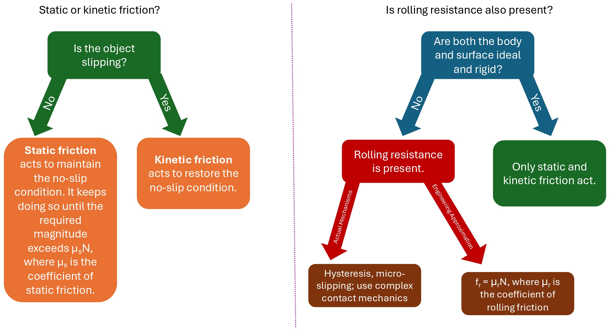Figure 5 | A flowchart to help students identify whether static friction, kinetic friction, and rolling resistance are present. When rolling resistance is present, the flowchart also distinguishes the differences between the underlying energy dissipation mechanism and the engineering approximation $f_r=\mu_r N$ .

Limitations

The analysis presented in this paper is intended as a pedagogical clarification of the forces involved in rolling motion rather than a comprehensive treatment of the physics of rolling motion. Multiple simplifying assumptions have been utilized to simplify and enhance the clarity of the distinctions between static friction, kinetic friction, and rolling resistance.

First, many of the examples assume rigid bodies rolling on rigid surfaces. This assumption removes the need to account for deformation, hysteresis, and other dissipative mechanisms, allowing static and kinetic friction to be analyzed independently of rolling resistance. While ideal rigid bodies do not exist in nature, this approximation is consistent with the idealized models commonly used in introductory physics classes to establish foundational principles before introducing real-world complications.

Second, the analysis of the rolling sphere in air uses low-Reynolds-number drag and rotational resistance models to illustrate the qualitative role of static friction during rolling. These expressions are intended as a qualitative model for this purpose. In addition, boundary effects and other more sophisticated interactions are beyond the scope of this work. Importantly, the central conceptual argument—that the contact force that acts is static friction while rolling without slipping—is based on the tendency-to-slip analysis and does not depend on the specific drag model employed.

Third, the discussion of rolling resistance focuses on the dominant physical mechanisms responsible for energy dissipation, including hysteresis, shifted normal-force distributions, and micro-slipping. These mechanisms are described qualitatively, and the paper does not attempt a quantitative analysis to describe rolling resistance for specific materials or operating conditions.

Finally, this work is primarily a conceptual pedagogical analysis. It does not include experimental measurements or classroom assessment of student learning.

Implications & Future Directions

We recommend that physics curricula clearly distinguish between the forces acting on a rigid body (static/kinetic friction) and the energy dissipation processes (rolling resistance) that occur in real, deformable systems, thereby providing students with a more accurate and coherent understanding of the world around them. For example, this paper could be used to help students understand the differences between static friction, kinetic friction, and rolling resistance. The examples discussed in this paper could be selectively incorporated into physics lessons. In addition, it could help to first introduce static and kinetic friction and their roles in rolling motion first, making sure that students fully understand them. Afterwards, rolling resistance could be discussed as a real-world phenomenon that only arises when the rigid body and surface assumptions are relaxed. Our future studies could help expand upon this paper by integrating the concepts in a lab²⁵^,²⁶^,²⁷, or could also evaluate the effectiveness of clarifying the differences between static friction, kinetic friction, and rolling resistance.

References

J. Walker, R. Resnick, & D. Halliday. Fundamentals of physics (10th ed.). Wiley. 2018. [↩] [↩]
H. D. Young, & R. A. Freedman. University physics (9th ed.). Addison-Wesley. 1996. [↩] [↩] [↩] [↩]
R. Rafika, & S. Syuhendri. Students’ misconceptions on rotational and rolling motions. Journal of Physics: Conference Series, Vol 1816., pg. 012016, 2021, https://doi.org/10.1088/1742-6596/1816/1/012016. [↩] [↩]
N. Demirci, I. Duman, & A. G. C. Sekercioglu. University students’ difficulties and misconceptions on rolling, rotational motion and torque concepts. International Journal on New Trends in Education and Their Implications, Vol 6., pg. 46, 2015. [↩]
C. Cari, P. Wulandari, N. Aminah, J. Handhika, & D. A. Nugraha. Students’ understanding level of friction force direction concept on rolling object. Journal of Physics: Conference Series, Vol 1153, pg. 012150, 2019, https://doi.org/10.1088/1742-6596/1153/1/012150. [↩]
E. Hasovic, V. Mesic, & N. Erceg. Conceptualizing Rolling Motion Through an Extreme Case Reasoning Approach. Phys. Teach., Vol 55, pg. 152, 2017, https://doi.org/10.1119/1.4976657. [↩]
A. Vidak, N. Erceg, E. Hasovic, S. Odzak, & V. Mesic. Teaching about rolling motion: exploring the effectiveness of an extreme case reasoning approach. J. Baltic Sci. Educ., Vol 17, pg. 511, 2018, https://doi.org/10.33225/jbse/18.17.511. [↩]
L. G. Rimoldini, & C. Singh. Student understanding of rotational and rolling motion concepts. Phys. Rev. Phys. Educ. Res., Vol 1, pg. 010102, 2005, https://doi.org/10.1103/PhysRevSTPER.1.010102. [↩] [↩]
K. Capell. Interesting results for rolling and slipping. Am. J. Phys., Vol 55, pg. 903, 1987, https://doi.org/10.1119/1.14950. [↩]
H. S. Kızılcık, M. Aygün, E. Şahin, N. Önder-Çelikkanlı, O. Türk, T. Taşkın, & B. Güneş. Possible misconceptions about solid friction. Physical Review Physics Education Research, Vol 17., pg. 023107, 2021, https://doi.org/10.1103/physrevphyseducres.17.023107. [↩] [↩]
A. D. Ambrosis, M. Malgieri, P. Mascheretti, & P. Onorato. Investigating the role of sliding friction in rolling motion: a teaching sequence based on experiments and simulations. European Journal of Physics, Vol 36., pg. 035020, 2015, https://doi.org/10.1088/0143-0807/36/3/035020. [↩] [↩] [↩]
R. D. Knight. Physics for scientists and engineers: a strategic approach. 4th ed. Pearson. 2017. [↩] [↩] [↩] [↩] [↩] [↩]
J. Hierrezuelo, & C. Carnero. Sliding and rolling: the physics of a rolling ball. Physics Education, Vol 30., pg. 177, 1995, https://doi.org/10.1088/0031-9120/30/3/009. [↩] [↩]
P. S. Carvalho, & A. S. Sousa. Rotation in secondary school: teaching the effects of frictional force. Physics Education, Vol 40., pg. 257, 2005, https://doi.org/10.1088/0031-9120/40/3/007. [↩]
C. W. Camp, & J. J. Clement. Preconceptions in mechanics: lessons dealing with students’ conceptual difficulties (2nd ed.). AIP Publishing. 2010. [↩]
D. R. Lide. CRC handbook of chemistry and physics (86th ed.). CRC Press. 2005. [↩] [↩]
G. K. Batchelor. An introduction to fluid dynamics. Cambridge University Press. 2000. [↩] [↩]
F. M. White. Fluid mechanics, 8th ed. McGraw-Hill Education. 2016. [↩]
L. D. Landau, & E. M. Lifshitz. Fluid mechanics (2nd ed.). Pergamon Press. 1987. [↩] [↩]
A. J. Goldman, R. G. Cox, & H. Brenner. Slow viscous motion of a sphere parallel to a plane wall—I Motion through a quiescent fluid. Chemical Engineering Science, Vol 22., pg. 637, 1967. [↩]
A. Salazar, A. Sanchez-Levega, & M. A. Arriandiaga. Is the frictional force always opposed to the motion?. Physics Education, Vol 25., pg. 82, 1990, https://doi.org/10.1088/0031-9120/25/2/001. [↩]
A. N. Gent, & J. D. Walter. The pneumatic tire. Mechanical Engineering Faculty Research. 2006. [↩] [↩]
C. E. Mungan. Rolling friction on a wheeled laboratory cart. Physics Education, Vol 47., pg. 288, 2012, https://doi.org/10.1088/0031-9120/47/3/288. [↩]
J. L. Johnson. Contact mechanics. Cambridge University Press. 2004. [↩]
L. Solvang, & J. Haglund. Learning with friction—students’ gestures and enactment in relation to a GeoGebra simulation. Res. Sci. Educ., Vol 52, pg. 1659, 2022, https://doi.org/10.1007/s11165-021-10017-7. [↩]
K. V. L. Maslova, B. de Jesus, & D. G. G. Sasaki. Understanding the effect of rolling friction in the inclined track experiment. Phys. Educ., Vol 55, pg. 055010, 2020, https://doi.org/10.1088/1361-6552/ab9217. [↩]
A. Suarez, D. Baccino, & A. C. Marti. An experiment to address conceptual difficulties in slipping and rolling problems. Phys. Educ., Vol 55, pg. 013002, 2020, https://doi.org/10.1088/1361-6552/ab4d1e. [↩]