Leveraging Contrast-Enhanced MRI Scans for Improved Alzheimer’s Diagnosis: A Deep Learning Approach

Abstract

The diagnosis of Alzheimer’s disease through MRI relies on large datasets, yet real clinical imaging data is limited because of cost, patient privacy, and variations in equipment quality. Contrast-enhanced MRI datasets provide a potential approach to alleviating data scarcity; however, their diagnostic capabilities remain uncertain. This paper studies the use of synthetically enhanced datasets, produced by tools such as CLAHE, Unsharp Masking, and Subtle Sharpening, for the detection of Alzheimer’s disease in MRI scans, ultimately comparing the diagnostic accuracy of models trained on real and synthesized datasets. Using a set of 8,000 brain scans (4,000 enhanced and 4,000 real) across four stages of Alzheimer’s progression, classical machine learning models and a convolutional neural network were trained and tested. They were then evaluated by comparing diagnostic accuracy, precision, recall, and F1-score. The CNN model achieved the best performance, reaching 0.7333 ± 0.0202 when trained on synthetic data, compared to 0.7381 ± 0.0280 when trained on real data. Considering CNNs are mainly used in image diagnosis, the results indicate high-quality image-enhanced data may support model training under controlled experimental conditions, although further validation is needed before it is integrated into medical applications. However, there runs a risk of new biases, such as feature amplification bias, where contrast and edge enhancements may amplify artificial patterns that do not correspond with disease-related biomarkers. Thus, more research should be done to further prove the validity of synthetic data for clinical use. These findings indicate synthesized datasets could be a viable option for widespread medical use.

Keywords: Machine learning (ML), Alzheimer’s disease, medical imaging, MRI contrast enhancement, CLAHE, biomarkers

Introduction

Using AI for medical diagnosis is revolutionizing healthcare; its increased accuracy and accessibility make for an increasingly effective diagnostic tool, specifically in medical imaging. Despite its transformative potential, this new sector of diagnostic medicine requires an exponential amount of data to train and test these models. This introduces problems such as data scarcity due to the cost of data, limited data for rare diseases, and ethical concerns regarding patient privacy. As a result, model training and generalization are hindered. Researchers have begun exploring synthetic datasets to fill in these data gaps. However, the reliability of these datasets in diagnostic treatment is not yet known. As a result, this project aims to measure performance when using synthetic datasets in medical imaging detection, using enhanced Alzheimer’s brain scan synthesized and non-synthesized datasets to test the reliability of using synthetic datasets in medical imaging. The evaluation of whether synthetic MRI datasets can provide reliable training data requires further validation.^1,2 This study evaluates whether models trained on synthetic MRI scans achieve comparable diagnostic performance to those trained on real MRI scans.

In this research, synthetic datasets are being used as well as real datasets to train and test each model. For the purpose of this study, the term synthetic datasets refers to the contrast-enhanced versions of existing MRI scans, not the generation of new images. The images are contrast-enhanced by CLAHE (Contrast Limited Adaptive Histogram Equalization), Unsharp Masking, and Subtle Sharpening. This is helpful in cases where the images are taken with old medical equipment or if the medical staff are inexperienced. Contrast sharpening is the most common method of enhancing image quality, so the efficiency of a correct diagnosis depends on the efficiency of the contrast enhancements. CLAHE is an image enhancement tool that improves contrast in medical imaging.³ It is the most popular spatial domain enhancement method because, unlike DCT and DWT, which work on the frequency components of the image, CLAHE improves local contrast by working in localized areas of the image. This results in a more accurate enhancement of the image’s important details while limiting noise. This is called spatial domain enhancement. Combining this method with other enhancing tools allows for improved usability for machine-learning classification while keeping the image’s most important components.^1,2 Synthetic datasets produced through contrast enhancement techniques such as CLAHE, Unsharp Masking, and Subtle Sharpening may provide additional data to support the training of Alzheimer’s classification models. However, their reliability needs careful and thorough evaluation.

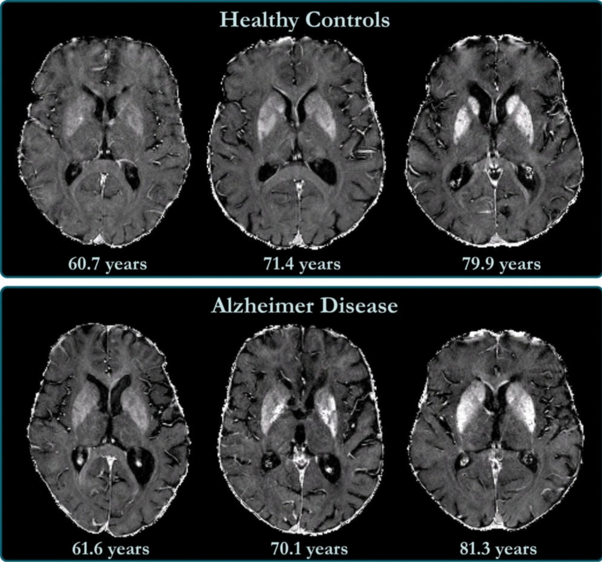
Alzheimer’s is a disease that affects memory and cognitive function; often, through medical imaging, the disease is diagnosed before the symptoms become too aggressive. Alzheimer’s is caused by a buildup of amyloid-β (Aβ) plaques and misfolded tau neurofibrillary tangles in the brain; someone who has Alzheimer’s has both of these proteins. The buildup of these proteins in the brain causes inflammation of brain tissue, loss of synapses, and disrupted neuron communication, eventually leading to neuron cell death. Neuron loss causes brain atrophy and hippocampal volume reduction; MRI scans detect these structural changes, which closely correlate with disease progression.^4,5,6,7 This is a disease that progresses slowly in elderly patients; diagnosing the disease early is beneficial as patients can receive better symptom management and support from their healthcare providers. This is why the dataset is split into four different classes depending on how far the disease has progressed. Additionally, machine learning is particularly useful in detecting early cases of Alzheimer’s.^8,9,10,11,12 Thus, there is a strong incentive to train models to accurately diagnose patients who are very mildly demented.

Synthetic datasets open up many opportunities, providing a solution to many of the data gaps seen in model testing today. A study by the Dundalk Institute of Technology tested the efficiency of using synthesized datasets to remove the bias minority patients face. They experience this bias because of a lack of data, creating a biased dataset. They found that “the effectiveness of synthetic data is closely dependent on the quality of the data generation process and the initial datasets used.”¹ Other studies reveal the importance of using both synthetic and real datasets to train AI; however, expert validation and balanced training approaches are still essential to creating the model.² Ultimately, although synthetic datasets provide a promising solution to overcome data limitations, they require careful validation and training to limit bias. For this reason, synthetic datasets are not widely used in medical applications despite rapid technological advancements. Furthermore, according to¹³ the model that achieved the best performance was K-nearest neighbor regression, achieving an accuracy of 97.33%. This model was trained on data from participants from the University of Washington’s Alzheimer’s Disease Research Center OASIS dataset. It was then cross-validated with the ADNI dataset, further confirming the effectiveness of this model.

In this field of study, there are many studies that focus solely on the performance of CNN models and their performance in diagnosing Alzheimer’s progression.^{14,15,11,16,17} However, this study aims to evaluate not only the performance of the CNN model but also classical models. Additionally, there are many studies that evaluate SVM or single ML models.^18,19 Therefore, this study will evaluate an ensemble model. Ensemble and multimodal learning approaches have shown strong performance in Alzheimer’s classification by combining diagnostic features and improving robustness.^20,21

Methods

Dataset

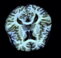
The dataset used is the Alzheimer’s Synthesized dataset on Kaggle, uploaded by Akmol Masud Ayon. The dataset consists of two components: normal and synthesised images. The normal images consist of 8000, carefully selected scans of the brain at 4 different stages of Alzheimer’s, Mild Demented, Moderate Demented, Non Demented, and Very Mild Demented. Furthermore the dataset is split so one half of the data is synthetic and the other half is real. The equal distribution of the data across the different stages facilitates unbiased model training. The synthesized dataset originates from the same base scan as the real dataset but is enhanced using a pseudo-RGB transformation which combines three image processing techniques. CLAHE (Contrast Limited Adaptive Histogram Equalization), Unsharp Masking, and Subtle Sharpening. CLAHE is a tool which improves the contrast locally, but it does not generate any new information, the case is the same with the other two tools, which amplify existing features but do not generate any new diagnostic data.³ The different colour channels in the synthesised images represent different enhancements made, allowing for new perspectives and connections to be made, by the model and researchers. More specifically it enhances subtle brain features which can signal Alzheimer’s disease. In order to protect patient privacy all images are anonymous. This dataset is a valuable recourse for training AI models for early detection and classification. The link to the data set is here: https://www.kaggle.com/datasets/masud1901/alzheimers-synthesized-dataset

Splitting the data

To evaluate the effect of synthetic data on the performance of these models, a combination of models were trained and tested. The tools used were os and path for file handling, cv2 and PIL.Image for image processing, and NumPy for mathematical operations and arrays, ultimately processing the data. Additionally, TensorFlow and scikit-learn were used for modeling, and scikit-learn was also used for evaluation. Secondly, the images were configured and processed. The original images had a resolution of approximately 200×190 pixels, with a range of 180–200 × 180–190. The images were resized using bilinear interpolation and normalized to the range [0,1]. Resizing ensured consistent input dimensions across models and reduced computational cost while preserving relevant anatomical features for classification. The random seed was set to 42 to ensure reproducibility of the data splits and model training. Next, the data was split into training and testing data: 67% training and 33% testing. This also ensured that randomness was consistent for each run through the seed that was set before. The classical machine learning models were then defined and trained. 33% was split into testing data because there needs to be a portion of the data on which the model is tested, but it is still a smaller percentage than the training data because more data is required for training than testing. Cross-validation was not used due to the large size of the dataset and computational constraints; however, to improve robustness, the CNN model was trained multiple times using different random seeds, and the mean accuracy and standard deviation were reported. The performance analyzed on the testing data is a good representation of the performance of the model on unseen cases.²²

Evaluation methods

In order to quantify the performance of the model, many classification evaluation metrics are used. The first is accuracy which is the measure of the difference between the correct predictions and the total number of predictions, the equation is Accuracy =TP+TNTP+TN+FN+FP. This is a very good metric to see how many predictions the model got correct, however can be misleading when data sets are unbalanced as the model may achieve high predictability by only predicting the highest class. This study however has a balanced dataset meaning that accuracy can be used as a good metric for measuring the efficiency of our models. Accuracy however does not distinguish between false positives and false negatives, for that reason precision, recall and F1-score were measured to provide a more complete evaluation of the model. Then precision is the measure of the accuracy of the positive predictions, the equation is Precision = TPTP+FP. This means a high precision means if the model predicts positive, it is likely to be correct. This is especially useful in situations where false positives are very costly, like in medical diagnoses or in spam detections. In contrast, Recall is a measure of how many of the positives was the model accurately able to predict, this is useful in situations where false negatives are costly, the equation is Recall = TPTP+FN. A middle ground for these two is an F1 Score. This is a combination of recall and precision meaning both metrics need to be high for the F1 Score to be high.  The equation is F1 = 2(PrecisionRecallPrecision + Recall).²³ Through these metrics the success of each model was measured.

Learning Algorithms

There are a variety of classical machine learning models used as well as one CNN model; this was done to cover a wide range of models with different features and advantages. Unlike convolutional neural networks, classical machine learning models do not preserve spatial relationships between pixels as a result of using flattened image vectors. Therefore, these models are not optimised for spatial feature learning, limiting their performance in medical imaging tasks such as MRI classification. Ultimately, the classical machine learning models provide a solid baseline for determining whether high performance is due to the synthetic data or the capabilities of each model.²⁴

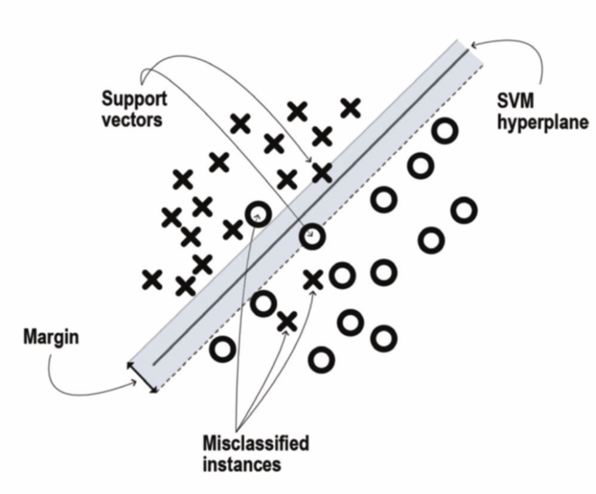
The first model is a Linear Support Vector Classifier (LinearSVC). The basis of the model is to split the data with a line of best fit, ultimately classifying the data. They are very effective in high-dimensional spaces, and are still effective when the number of features is much greater than the number of samples, which is true in this case as we are working with image features. They work very efficiently without using excessive memory and serve as a very useful baseline model, assisting in the evaluation of more complex models, as they should be working better than simple linear separation. However, the linear separation fails to take into account the complex non-linear features in the images. This results in image quality being somewhat unimportant in the overall accuracy of the model.²⁴

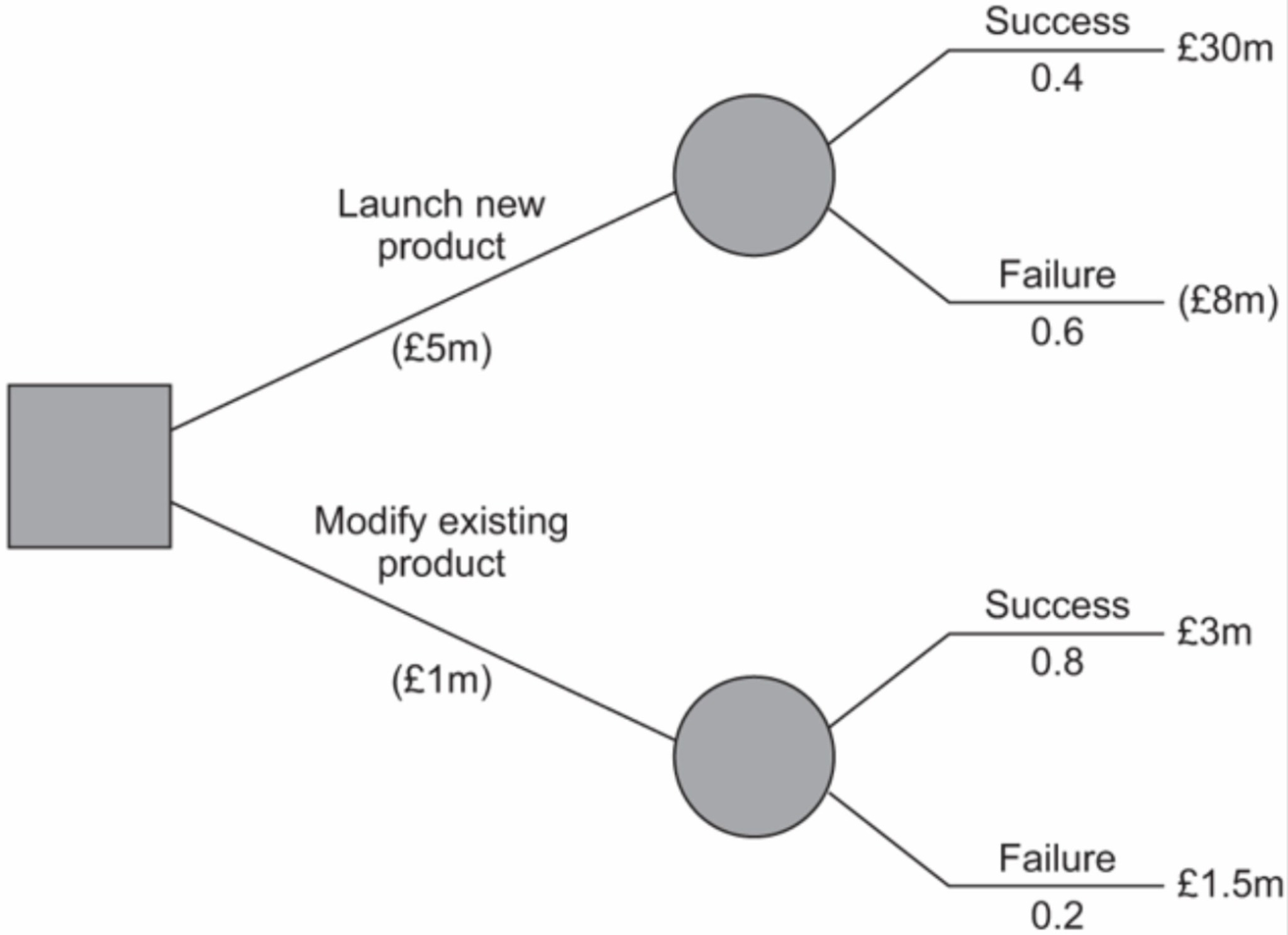
The second model, the Decision Trees model, is a non-parametric supervised learning method. The model learns to make certain if-then-else decision rules and classifies the data. The advantages of decision trees are that they require little data interpretation and data processing, as well as having an intuitive structure. It handles numerical data such as pixel intensity well and can capture non-linear patterns in the data. However, it is very prone to overfitting and is generally very unstable, as small changes in data can produce very different trees. Additionally, the predictions are stepwise and may not account for subtle gradients in imaging data. It can also become biased towards dominant classes, such as skewed Alzheimer’s severity classes. This may require managing the dataset’s balance and using ensembles like Random Forests for stability and improved performance.²⁴

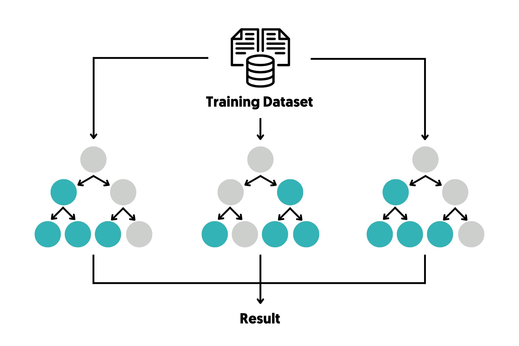
The third model, the Random Forest model, builds multiple decision trees during training and combines their outputs. This results in more accurate and stable predictions; for classification, the result is decided by majority voting among the trees. The advantages are that the model is highly accurate, as it is robust to noise and outliers. It also identifies specific features and identifies which ones are most important for image classification. However, it has a risk of overfitting and a slower prediction time.²⁴

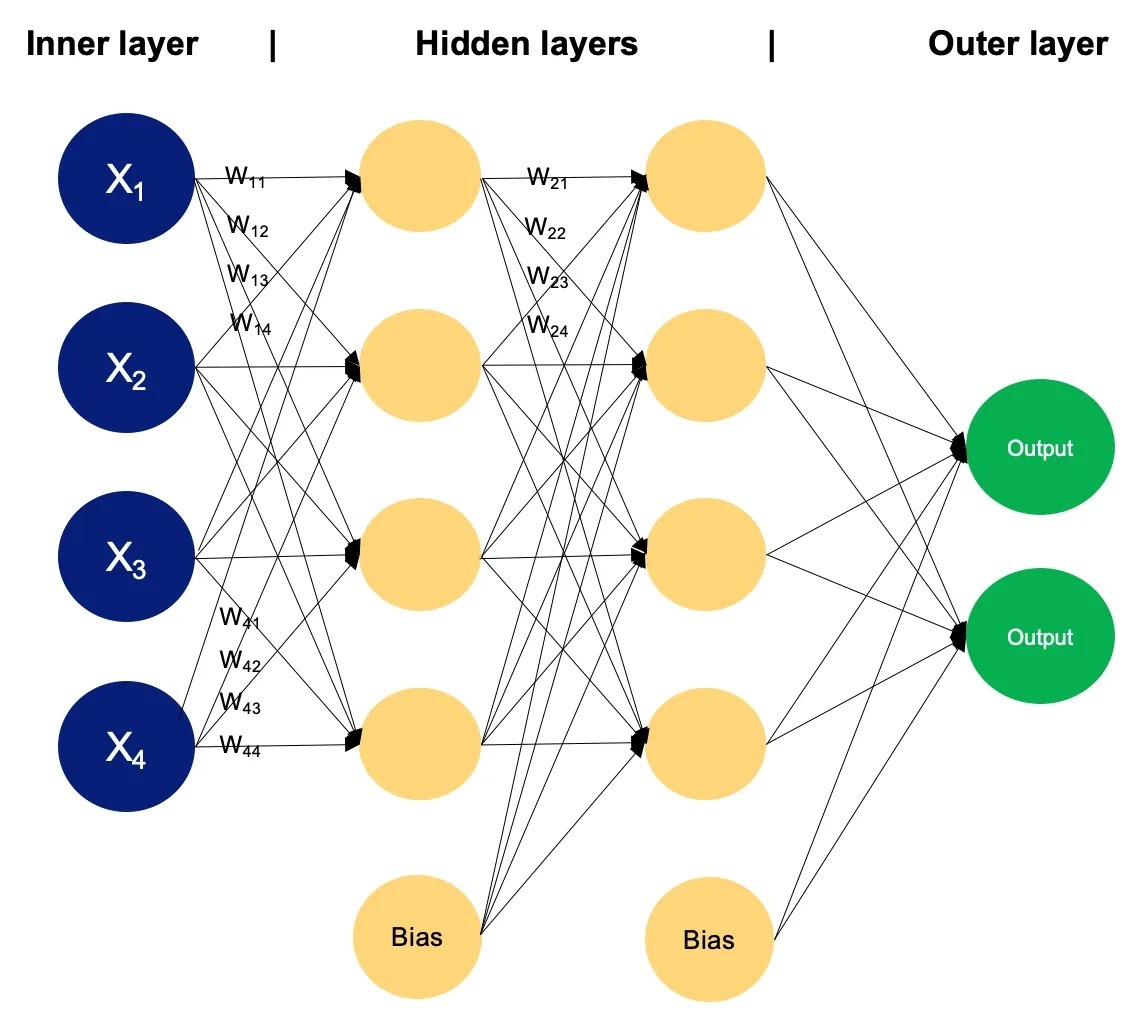
The fourth model, Multi-Layer Perceptrons (MLPs), are the simplest of neural networks which, as the name implies, have layers of “neurons” that have specific parameters. With many layers of neurons, the model is able to identify very complex patterns, specifically non-linear relationships between features; however, it does not explicitly capture spatial structure in image data. Additionally, it is sensitive to scaling, so proper normalisation of input features is crucial for training stability.^25,26

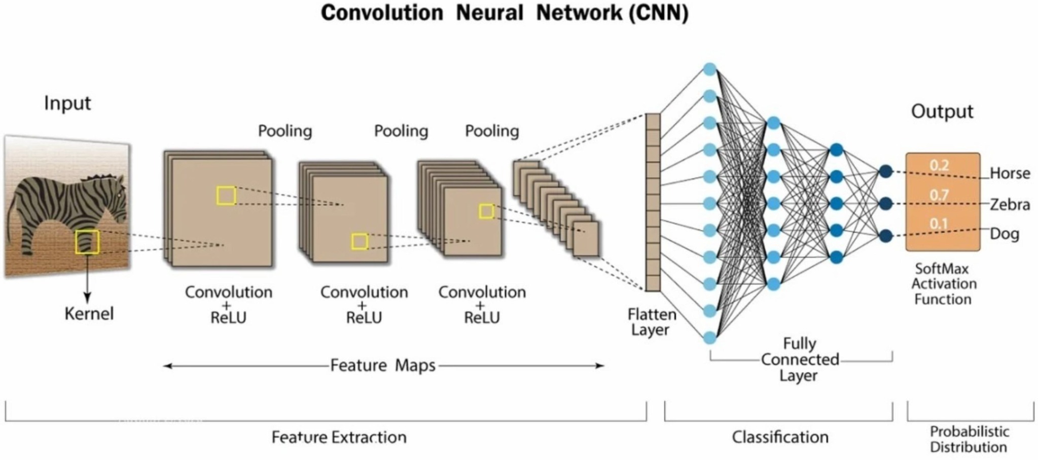
The final model is a Convolutional Neural Network (CNN). CNNs are a type of neural network that use convolutional filters to learn specific spatial features. This makes it very effective for visual recognition. Specifically, it is able to learn patterns such as edges, shapes, and textures, and is therefore able to make more precise predictions from images such as MRI scans. What differentiates CNNs from other neural networks are the hidden convolutional layers, which are what allow the model to detect and extract hierarchical patterns from data. Convolutional layers have neurons that have a local receptive field, meaning they look at a specific part of the image, being able to recognise localised patterns. This is unlike fully connected layers, which process the whole image as a vector, not looking at localised regions, with no context with each other. Secondly, each convolutional layer has a series of filters called kernels, which are what detect each feature. Finally, after the filters are applied over the input, an activation function is applied; in this case, it is the Rectified Linear Unit function. According to a literature review by Ebrahimighahnavieh et al., ReLU is the most widely used activation function for CNN studies. There are also max-pooling layers in this model, which shrink the image while keeping the most prominent features in the data. This helps magnify the most prominent features in the images while also keeping the image size smaller to maximise efficiency. The flattening layer acts to convert the output from a multi-dimensional tensor to one dimension so it can be processed by the final dense layers. The dense layers act as the final classification of the data, using the non-linear features extracted to classify each scan.^25,26

CNNs are trained through supervised learning, where all the data has been previously labeled. First, a forward pass involves inputting the data through the model, then the loss is calculated. The loss function used is cross-entropy. The gradient of the loss function is calculated with respect to the weights of each layer. Adam, an optimiser, uses those gradients to update the weights of the model through a process called backpropagation. This is done through many epochs until the loss is minimised. Additionally, there runs a risk of overfitting; to prevent this, CNNs train on very large datasets. Hence, there is a need for more augmented data such as synthetic datasets, additionally highlighting the importance of measuring the reliability of such synthetic data.^25,26

The CNN model in this study used two convolutional layers. The layers used 32 and 64 filters, as well as a 3×3 kernel. Then, they were each followed by 2×2 max-pooling, and, on top of that, a flattening layer. Then, a dense layer with 64 units and a softmax output layer with four classes was used. The optimiser used was the Adam optimiser with a learning rate of 0.001. The loss function used was sparse categorical cross-entropy loss, which is often used for situations where each image belongs to only one class. The models were trained for up to 30 epochs with a batch size of 32, using a 20% validation split. After that, early stopping was used to reduce overfitting. It had a patience of 3 and used restoring best weights. The model was trained 5 times with a different seed applied each time, and mean accuracy and standard deviation were reported to measure performance variability throughout the runs.^25,26

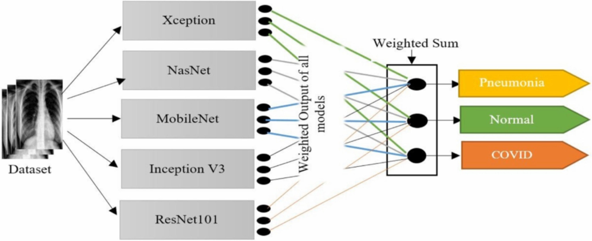
After testing the performance of each individual model, it became clear each has their own strengths and limitations; for this reason, an ensemble approach was explored, aiming to reduce bias and improve generalisation across unseen data. An ensemble model is a model that combines multiple models to achieve more accurate predictions. While single models have biases and weaknesses, pooling the models’ results can reduce generalisation error and improve robustness. In traditional ensemble models, an equal majority vote is taken to get the predictions, meaning each model has equal priority. However, this does not account for the varying strengths of each of the models; therefore, using a weighted average instead of a simple average is often more accurate. A weighted average prioritises more accurate or reliable models, as the weights are assigned to each model based on their accuracy. The reason this is done is because the higher the accuracy, it proves the validity of each model.²⁷

Results

Model	Real	Synthetic
Linear SVC	0.6246	0.6424
Decision Tree	0.4856	0.4879
Random Forest	0.3602	0.3655
MLP	0.6500	0.6436
CNN	0.7381	0.7333
Ensemble	0.7280	0.7258

The CNN model achieved the highest accuracy with both real and synthetic data, with 0.7381 and 0.7333 respectively. The difference between these two results is less than 1%. This similar accuracy between real and synthetic datasets implies that synthetic datasets do not distort anatomical features related to Alzheimer’s disease diagnosis. This effect is similarly seen amongst studies with other synthetic data enhancement methods, such as Rezaei and Fathi (2024), who used GAN-enhanced images to improve CNN classification accuracy.²⁸

The classical machine learning models achieved lower accuracies and showed little variation between real and synthetic data. This is because these models flatten image vectors and are therefore not optimised for spatial feature learning. The CNN, on the other hand, is optimised for spatial feature learning, so it can identify anatomical features in MRI scans.^25,26

Real Data

Linear SVC	Precision	Recall	F1-score
0	0.61	0.60	0.61
1	0.82	0.77	0.79
2	0.56	0.63	0.59
3	0.53	0.50	0.52

Decision Tree	Precision	Recall	F1-score
0	0.42	0.42	0.42
1	0.64	0.65	0.64
2	0.51	0.47	0.49
3	0.38	0.40	0.39

Random Forest	Precision	Recall	F1-score
0	0.25	0.22	0.23
1	0.38	0.82	0.52
2	0.44	0.39	0.42
3	0.15	0.01	0.01

MLP	Precision	Recall	F1-score
0	0.00	0.00	0.00
1	0.25	1.00	0.40
2	0.00	0.00	0.00
3	0.00	0.00	0.00

CNN	Precision	Recall	F1-score
0	0.72	0.75	0.74
1	0.93	0.97	0.95
2	0.75	0.72	0.74
3	0.65	0.63	0.64

Ensemble	Precision	Recall	F1-score
0	0.71	0.69	0.70
1	0.89	0.94	0.91
2	0.72	0.70	0.71
3	0.59	0.58	0.59

When trained on real data, the CNN achieved the highest performance, as it had the highest precision, recall, and F1-scores across all Alzheimer’s stages. The ensemble model was the next best-performing model but was still strong overall, along with the Linear SVC, which showed moderate performance. Finally, the poorest-performing models were the Decision Tree and Random Forest, and notably, the MLP failed to reliably classify most classes.

Synthetic Data

LinearSVC	Precision	Recall	F1-score
0	0.61	0.67	0.64
1	0.79	0.81	0.80
2	0.61	0.61	0.61
3	0.55	0.48	0.51

Decision Tree	Precision	Recall	F1-score
0	0.45	0.43	0.45
1	0.60	0.63	0.61
2	0.47	0.47	0.47
3	0.41	0.42	0.32

Random Forest	Precision	Recall	F1-score
0	0.26	0.29	0.27
1	0.39	0.79	0.53
2	0.44	0.37	0.40
3	0.50	0.00	0.01

MLP	Precision	Recall	F1-score
0	0.69	0.57	0.62
1	0.82	0.83	0.82
2	0.57	0.68	0.62
3	0.52	0.49	0.50

CNN	Precision	Recall	F1-score
0	0.76	0.74	0.75
1	0.94	0.97	0.95
2	0.75	0.68	0.71
3	0.63	0.68	0.65

Ensemble	Precision	Recall	F1-score
0	0.73	0.68	0.70
1	0.87	0.92	0.89
2	0.68	0.70	0.69
3	0.61	0.60	0.61

When trained on synthetic data, the CNN performed the best, with high precision, recall, and F1-scores across all classes. The next best were the Ensemble model and Linear SVC, which performed well. Interestingly, the MLP greatly improved its performance compared to the real data. Finally, the Decision Tree and Random Forest remained relatively weak, particularly when classifying later Alzheimer’s stages.

Discussion

The model with the best performance was the CNN, with an accuracy of 0.7333 when trained on real data and also had the best performance when trained on synthetic data with an accuracy of 0.7333. This research demonstrated that, under controlled conditions, training CNN models on synthetic datasets and real datasets produce comparable results with only a standard deviation of ±0.0202 and ±0.0280 respectively. These results suggest that synthetic MRI data can support model training for diagnostic classification tasks. However there are still limitations to this research. For instance, the model performance was evaluated on a single dataset. Synthetic data and real datasets were compared under controlled conditions, however the models were not tested on external MRI datasets. This demonstrates that the generalization of these findings to real clinical environments cannot be proved.^1,2 The enhancement methods do not create any new information, instead highlighting important features, this creates a potential for overfitting and bias in diagnosis.³ However, there is no limitation to using a combination of synthetic and real data which reveals the possibility of improving diagnosis and hence, alleviating data scarcity amongst medical scans.^1,29 Ultimately, the results suggest that synthetic data may be a viable alternative for training CNN models.

The results and limitations of this study provoke a series of extended questions. To what extent do models trained purely on synthetic data perform when applied to varied sources of real imagery, such as different scanner types? Does synthetic data amplify non disease features leading to misdiagnosis? Besides Alzheimer imaging, how may this research extend to other medical fields such as ultrasound or cardiac MRI, and how can this extend beyond classification, into treatment planning? What precautions must be taken to validate synthetic data as a medical tool for classification?  Future work should additionally evaluate synthetic trained models on real external datasets. Further investigation into these questions will help validate and integrate the use of synthetic data with rigorous demands of clinical practice, ensuring the safety and reliability of AI tools using synthetic data.³⁰

Acknowledgements

The author acknowledges Odysseas Drosis for mentorship and feedback that supported the development of this paper. The author additionally acknowledges Akmol Masud Ayon for providing the dataset on Kaggle. No external funding was used for this research.

References

1. A. M. Ayon, S. Patel, R. Singh. Synthetic versus real MRI data for Alzheimer’s detection using CNN-based classifiers. Frontiers in Computational Neuroscience. Vol. 17, pg. 9931305, 2023, https://doi.org/10.3389/fncom.2023.9931305. [↩] [↩] [↩] [↩] [↩]
2. J. C. Moreno-Tagle, J. Olveres, B. Escalante-Ramírez. Synthetic versus real: Exploring the impact of synthetic data on medical image classification. Proceedings of SPIE. Vol. 12998, 2023, https://doi.org/10.1117/12.3022261. [↩] [↩] [↩] [↩]
3. S. M. Pizer, E. P. Amburn, J. D. Austin, et al. Adaptive histogram equalization and its variations. Computer Vision, Graphics, and Image Processing. Vol. 39, No. 3, pg. 355-368, 1987. [↩] [↩] [↩]
4. O. Colliot, C. Klöppel, C. Stonnington, B. Draganski, C. Chu, J. D. Rohrer, N. C. Fox, J. Ashburner, R. S. J. Frackowiak. Discrimination between Alzheimer disease, mild cognitive impairment, and healthy controls using automatic classification of brain MRI. Radiology. Vol. 248, pg. 194–201, 2008, https://doi.org/10.1148/radiol.2481071106. [↩]
5. C. Plant, S. J. Teipel, A. Oswald, T. Böhm, T. Meindl, J. Mourao-Miranda, H. Hampel, M. Ewers. Automated detection of brain atrophy patterns based on MRI for the prediction of Alzheimer’s disease. NeuroImage. Vol. 50, pg. 162–174, 2010, https://doi.org/10.1016/j.neuroimage.2009.11.046. [↩]
6. M. Dyrba, M. Grothe, S. J. Teipel. Multiclass pattern recognition for detecting Alzheimer’s disease and mild cognitive impairment using MRI. NeuroImage. Vol. 56, pg. 212–221, 2011, https://doi.org/10.1016/j.neuroimage.2011.01.008. [↩]
7. H. Tong, R. Wolz, P. Coupé, J. V. Hajnal, D. Rueckert. Segmentation of MR images via discriminative dictionary learning and sparse coding: Application to hippocampus labeling. NeuroImage. Vol. 76, pg. 11–23, 2013, https://doi.org/10.1016/j.neuroimage.2013.02.069. [↩]
8. G. Basaia, F. Agosta, L. Wagner, E. Canu, S. Magnani, R. Santangelo, M. Filippi. Automated classification of Alzheimer’s disease and mild cognitive impairment using a single MRI and deep neural networks. NeuroImage: Clinical. Vol. 21, pg. 101645, 2019, https://doi.org/10.1016/j.nicl.2018.101645. [↩]
9. A. Farooq, S. Anwar, M. Awais, S. Rehman. A deep CNN based multi-class classification of Alzheimer’s disease using MRI. Neurocomputing. Vol. 282, pg. 248–257, 2018, https://doi.org/10.1016/j.neucom.2017.08.093. [↩]
10. S. Sarraf, G. Tofighi. DeepAD: Alzheimer’s disease classification via deep convolutional neural networks using MRI and fMRI. Frontiers in Neuroscience. Vol. 11, pg. 1–12, 2017, https://doi.org/10.3389/fnins.2017.00037. [↩]
11. Y. Liu, M. Xu, C. Zhang. Multi-stage Alzheimer’s disease classification using structural MRI and deep learning. Scientific Reports. Vol. 11, pg. 12839, 2021, https://doi.org/10.1038/s41598-021-92395-4. [↩] [↩]
12. E. Hosseini-Asl, J. Gimel’farb, A. El-Baz. Alzheimer’s disease diagnostics by adaptation of 3D convolutional network. Proceedings of IEEE International Conference on Image Processing. pg. 126–130, 2016, https://doi.org/10.1109/ICIP.2016.7532332. [↩]
13. H. Aslan, A. Yildirim Özüpak. Machine learning-based classification of Alzheimer’s disease using MRI data. Diagnostics. Vol. 14, 2024, https://doi.org/10.3390/diagnostics14010092. [↩]
14. H. Korolev, A. Safiullin, M. Belyaev, Y. Dodonova. Residual and plain convolutional neural networks for 3D brain MRI classification. Computerized Medical Imaging and Graphics. Vol. 61, pg. 75–82, 2017, https://doi.org/10.1016/j.compmedimag.2017.07.008. [↩]
15. R. Katabathula, J. Wang, R. Prasanna. Predict Alzheimer’s disease using hippocampus MRI data: A lightweight 3D deep convolutional network model with visual and global shape representations. IEEE Access. Vol. 9, pg. 59332–59345, 2021, https://doi.org/10.1109/ACCESS.2021.3073116. [↩]
16. X. Jiang, Y. Wang, X. Chen. Alzheimer’s disease neuroimaging classification using deep convolutional neural networks. Frontiers in Neuroscience. Vol. 16, pg. 834271, 2022, https://doi.org/10.3389/fnins.2022.834271. [↩]
17. S. Lu, X. Lu, Y. Lin, X. Zhang. Alzheimer’s disease classification using deep learning with structural MRI data. IEEE Journal of Biomedical and Health Informatics. Vol. 25, pg. 1737–1746, 2021, https://doi.org/10.1109/JBHI.2020.3033072. [↩]
18. C. Klöppel, C. M. Stonnington, C. Chu, B. Draganski, R. I. Scahill, J. D. Rohrer, N. C. Fox, J. Ashburner, R. S. J. Frackowiak. Automatic classification of MR scans in Alzheimer’s disease. Brain. Vol. 131, pg. 681–689, 2008, https://doi.org/10.1093/brain/awm319. [↩]
19. I. Magnin, S. Mesrob, S. Kinkingnéhun, M. Pélégrini-Issac, O. Colliot, M. Sarazin, B. Dubois, S. Lehéricy, H. Benali. Support vector machine-based classification of Alzheimer’s disease from whole-brain anatomical MRI. Neuroradiology. Vol. 51, pg. 73–83, 2009, https://doi.org/10.1007/s00234-008-0463-x. [↩]
20. H. Suk, S. Lee, D. Shen. Deep ensemble learning of sparse regression models for brain disease diagnosis. Medical Image Analysis. Vol. 37, pg. 101–113, 2017, https://doi.org/10.1016/j.media.2017.01.008. [↩]
21. D. Zhang, Y. Wang, L. Zhou, H. Yuan, D. Shen. Multimodal classification of Alzheimer’s disease and mild cognitive impairment. NeuroImage. Vol. 55, pg. 856–867, 2011, https://doi.org/10.1016/j.neuroimage.2011.01.008. [↩]
22. R. Kohavi. A study of cross-validation and bootstrap for accuracy estimation and model selection. IJCAI. Vol. 14, No. 2, pg. 1137–1145, 1995. [↩]
23. M. Sokolova, G. Lapalme. A systematic analysis of performance measures for classification tasks. Information Processing & Management. Vol. 45, No. 4, pg. 427–437, 2009. [↩]
24. T. Hastie, R. Tibshirani, J. Friedman. The Elements of Statistical Learning: Data Mining, Inference and Prediction (2nd ed.). Springer, 2009. [↩] [↩] [↩] [↩]
25. Y. Guo, Y. Liu, A. Oerlemans, S. Lao, S. Wu, M. S. Lew. Deep learning for visual understanding: A review. Neurocomputing. Vol. 187, pg. 27–48, 2016, https://doi.org/10.1016/j.neucom.2015.09.116. [↩] [↩] [↩] [↩] [↩]
26. A. Ebrahimighahnavieh, S. Luo, R. Chiong. Deep learning to detect Alzheimer’s disease from neuroimaging: a systematic literature review. Computer Methods and Programs in Biomedicine. Vol. 187, pg. 105242, 2020, https://doi.org/10.1016/j.cmpb.2019.105242. [↩] [↩] [↩] [↩] [↩]
27. T. G. Dietterich. Ensemble methods in machine learning. Multiple Classifier Systems. Vol. 1857, pg. 1-15, 2000. [↩]
28. A. Rezaei, M. Fathi. Enhancing Alzheimer’s disease prediction: a novel approach to leveraging GAN-augmented data for improved CNN model accuracy. arXiv preprint. 2024, https://arxiv.org/pdf/2409.02961. [↩]
29. J. C. Moreno-Tagle, J. Olveres, B. Escalante-Ramírez. Synthetic versus real: Exploring the impact of synthetic data on medical image classification. Proceedings of SPIE. Vol. 12998, 2023, https://doi.org/10.1117/12.3022261. [↩]
30. A. Vabalas, E. Gowen, E. Poliakoff, A. J. Casson. Machine learning algorithm validation with a limited sample size. PLoS ONE. Vol. 14, No. 11, e0224365, 2019. [↩]