

Abstract
Existing models of auditory roughness predict that the minor third is rougher than the major third. This difference is evident in simple tones and controlled chords, but in complex recordings it is nearly absent. In this paper, I use 18,486 recordings from the MTG-Jamendo dataset to explore why this is the case. Decomposing total roughness by frequency separation shows offsetting effects of different sets of frequency pairs. Recordings that are minor-like have a larger number of pairs at frequency separations associated with roughness. Major-like recordings tend to have a more even distribution of amplitude across the most salient spectral peaks. The more balanced amplitudes increase the average pairwise contribution in major-like recordings, partly offsetting the larger number of relevant pairs in minor-like recordings. To assess the relevance of amplitude distribution, I equalize the amplitudes of the selected spectral peaks while holding their frequencies and total energy fixed. The simulated difference in roughness increases in the expected direction, with minor-like recordings showing greater roughness than major-like recordings in all eight frequency-separation categories. The major–minor roughness difference persists as spectral complexity increases if the added frequencies retain their harmonic structure. The recovered roughness pattern does not significantly predict happy–sad expression after accounting for mode. The paper argues that the difference in total roughness between major-like and minor-like recordings is small partly because opposing spectral contributions cancel each other out.
Introduction
Major- and minor-mode music is often associated with different emotions. Major-mode compositions are often described as brighter, minor-mode compositions as darker1,2. One contributor to these associations is roughness, which is caused by rapid amplitude fluctuation due to frequency interference. Roughness contributes to dissonance3,4 and aversive responses5,6. Computational simulations indicate that minor thirds, when presented as isolated intervals, sound rougher than major thirds. This difference is still present in synthetic triads with harmonic partials7,8, but perceived dissonance varies with musical genre and listener skill9, and real music is far more complex than isolated intervals. Real music has frequencies overlapping from different instruments, percussion and production elements. Current models evaluate the interactions of frequencies and sum them to determine the overall roughness. What about the major–minor roughness difference in real music?
Using 18,486 recordings from the MTG-Jamendo dataset and controlled synthetic experiments, I examine why the minor-rougher difference nearly disappears in real music. I find that contributions from different frequency-separation ranges partly cancel each other. Minor-like recordings have slightly more pairs in roughness-relevant ranges, but major-like recordings have more balanced amplitudes, increasing the average roughness contribution of each pair. When I equalize the amplitudes of retained spectral peaks, the minor-rougher difference becomes larger. Synthetic experiments also show that the difference persists as more frequencies are added, provided they retain harmonic structure.
Previous studies show that roughness depends on spacing and amplitudes of frequency components4,7. Roughness is an interaction among nearby frequencies. Harmonicity is the frequency structure of a sound10,11. Both roughness and harmonicity determine how consonant a sound is perceived, but musical experience and cultural background also play a role12,13,14. Judgments of consonance also depend on timbre and harmonic structure15,16,17. Previous studies have demonstrated acoustic differences between major and minor mode music18,19,20. Computational approaches have been used to explore the relationship between roughness and harmonicity and tonal organization21,22. However, little attention has been given to how frequency spacing and amplitude distribution may offset each other.
Roughness is only one aspect of consonance and musical expression. Another aspect that contributes to the shaping of tonal organization is harmonicity11. Major-minor emotional contrasts rely on timbre, tempo and other psychological factors23,24,25. Controlling for mode, the pattern of roughness contributions across frequency ranges does not significantly predict happy-sad expression. Differences in roughness are hard to detect in complex recordings, where the opposing frequency pairs cancel each other.
I test the following five predictions. First, I expect the minor-rougher difference to become smaller as more frequencies are added. Second, I test whether the small difference in total roughness results from cancellation across frequency ranges. Third, I examine whether the effect of frequency arrangement on total roughness is in the opposite direction to that of the amplitude distribution. Fourth, equalizing peak amplitudes within the model increases the minor-rougher difference. Fifth, the minor-rougher contrast is better preserved in more harmonically organized spectra.
Acoustic Background
Musical sounds usually contain many frequencies. A played or sung note contains a fundamental and higher-frequency partials; a chord brings together the partials of several notes. If two components are close in frequency, their interaction leads to fluctuations in amplitude, called beating. Very close frequencies produce slow beats. As the separation increases, the beats become faster and may be heard as roughness3,4,1. Roughness is strongest at intermediate separations. Farther apart, the components become easier for the auditory system to distinguish, and roughness decreases.
Frequency separation cannot be described well by a fixed number of hertz. Auditory frequency resolution changes across the spectrum. This is commonly described in terms of critical bandwidth. So, the same spacing in hertz can produce different interactions at low and high registers. My analysis spans different notes, instruments, and registers, so I need to account for this variation.
Sethares7 expressed the dependence of pairwise roughness on frequency separation and amplitude computationally for two spectral peaks with frequencies f1 and f2 (in Hz) and amplitudes A1 and A2. In this study, peak amplitudes are the absolute values of the short-time Fourier transform (STFT) coefficients, expressed on a linear scale:
where
The term in brackets in Eq (1) is the roughness kernel. It measures the contribution of a pair as a function of its frequency separation. If the two frequencies are close, the kernel is small. It rises over a moderate range and then decreases as the elements become more easily distinguishable. The term w(A1, A2) is a measure of how strong the influence of the amplitudes is on the interaction. Following Sethares, I use w = min(A1, A2). For a sensitivity check, I also use product weighting, w = A1A226. The numerical estimates and possibly the observed patterns are model dependent, since different alternative roughness models exhibit differences in frequency separation and amplitude27,8. I use the Sethares formulation because it has a clear pairwise structure which makes the frequency-separation decomposition used in this paper easier to perform.
The minimum amplitude weighting has important implications. A pair is only strong when both parts are strong. Therefore, if one element is missing, it limits the input of both. Different distributions of the amplitude between the spectral peaks cause two spectra with the same frequency locations and the same total amplitude to have different roughness values.
For a complex spectrum, total roughness is the sum of the contributions from all unique pairs of spectral peaks:
I call this total roughness. Total roughness aggregates interactions across notes and harmonics and sound sources. I differentiate between frequency arrangement (distribution of pairs over separation intervals) and spectral amplitude distribution (weights assigned to those interactions). The analyses investigate whether aggregation masks mode-related differences in these components.
Roughness is different from harmonicity. Harmonicity is a measure of how closely the spectral components follow a harmonic series. Roughness arises from interactions between neighboring frequencies26,11. Both can enhance harmony. But they describe different properties of sound28,29,30. Therefore I will use metrics of harmonic and tonal structure in the subsequent analyses as a proxy for harmonicity rather than roughness.
Methods
Data and Acoustic Measures
I use the MTG-Jamendo dataset31, consisting of 55,609 Creative Commons tracks by independent musicians from various genres. Of these, 54,080 recordings have extractable audio and are used for the replication analyses reported in Supplement Section S8. The main analyses are based on the 18,486 tracks that have at least one mood/theme label.
For the secondary analysis of happiness and sadness, I have a collection of 2,376 tracks from 402 different artists that are labeled only as “happy” or “sad” (1,642 happy and 734 sad). The tags assigned by the uploader are interpreted as idiosyncratic expression of emotion, rather than any normative judgment of perceived or felt emotion32,33. The happy–sad classification models also take into account root-mean-square (RMS) signal level, spectral flux, onset rate, and tempo.
Supplementary Table S7 compares nine acoustic attributes across the mode-quartile categories, with small standardized differences for all recorded features (|d| ≤ 0.11). The genres of the groups are different: pop music is more frequent in major-like tracks (21%) than in minor-like tracks (11%), while electronic music is more frequent in minor-like tracks (29%) than in major-like tracks (19%).
When available, I use the lower bitrate full-track audio from MTG-Jamendo, otherwise the corresponding full quality file. I analyze up to the first 30 seconds of every recording. This provides a reproducible sampling rule and common analysis length for recordings of 30s minimum. The verified MTG-Jamendo preview files are mono, so that step of the mono conversion does not affect those files.
I resample the audio to 22,050 Hz. I use librosa 0.11.034 for the extraction of acoustic features and scikit-learn 1.3.0 for the classification35. The script is executed in Python 3.11.5 using NumPy 1.26.4 and SciPy 1.11.3.
To study the temporal variations in frequencies, I split the audio into overlapping segments. Each frame consists of 2048 samples, i.e. about 93 ms, and the next frame starts 512 samples later. I use a Hann window and compute the short-time Fourier transform with a Fast Fourier Transform length of 2,048. This gives a frequency bin spacing of roughly 10.77 Hz.
For each frame, I use scipy.signal.find_peaks to find local maxima in the magnitude spectrum. A peak must be greater than 1% of the maximum magnitude in that frame and occur at a frequency of at least 20 Hz. If there are more than 15 peaks satisfying these criteria, the 15 strongest ones will be kept. Otherwise, I keep all qualifying peaks. I then compute roughness from pairs of preserved peaks. When there are 15 peaks, there are 105 possible pairs. If a frame has fewer than two peaks, then there are no pairs and hence the roughness is zero for that frame. These frames are still included in the calculation of my average.
For each retained pair, I use the Sethares roughness model (Eq (1)), add the contributions for each frame, and average the frame-level sums over 100 uniformly sampled frames to obtain one roughness value for the track. Frame selection is deterministic using np.linspace with dtype=int and does not involve any random sampling. In the frequency-separation decomposition, frames with fewer than two retained peaks are discarded in the averaging. In a review of 500 tracks, 0.8% of frames have fewer than two retained peaks. The two averaging methods differ by less than 1% in the mean at the track level. No explicit minimum-distance constraint is applied between peaks. I provide a sensitivity analysis with a minimum peak separation of three bins (~32.3 Hz) in the Supplemental Appendix.
Moreover, I use level-normalized roughness, because roughness depends on the signal amplitude. Roughness is computed by dividing by the RMS signal level for minimum amplitude weighting and by the square of the RMS for product weighting.
I classify major and minor tonality based on the chroma profile of each track, a representation of the relative intensity of the 12 pitch classes, irrespective of octave. Following Krumhansl36, I correlate the chroma profile of each track with reference profiles for all 12 major and minor keys. The mode score is determined by the difference between the largest major-key correlation and the largest minor-key correlation. Positive values indicate a major-like structure and negative values indicate a minor-like structure. I use a continuous score, because actual performances may modulate or combine major and minor qualities. Because the reference profiles are based on Western tonal evaluations, the mode score is an imperfect proxy for musical mode. The key confidence of each track is defined by the highest correlation with any of the 24 Krumhansl key profiles. It measures the robustness of the optimal key-profile alignment instead of the distinctiveness of the deduced key. Both the mode score and the roughness are computed from the same audio, which suggests that they might be related through overlapping spectral data, although they represent different characteristics: the energy distribution across pitch classes and the interactions between spectral peaks, respectively.
The Krumhansl classifications are compared to those obtained from the principal profiles of Temperley37 and Aarden38. Krumhansl agrees with the three-method majority-vote consensus on 90% of mode-quartile tracks (κ = 0.79). Krumhansl adds to that vote. So this agreement is a consistency measure across methods, not independent validation. Keeping only those tracks for which all three methods agree leaves 66% of the quartile sample. Minor-like tracks are slightly rougher in this subset (d = +0.08, 95% CI [−0.01, +0.16]). The predicted difference is larger than for the first quartile sample (d = +0.03), but still small.
The exhaustive feature extraction resulted in 29 acoustic attributes. The main analysis uses three measures of tonal and spectral organization: peak harmonicity, harmonic ratio, and spectral flatness. Peak harmonicity is a measure of the degree to which the dominant spectral peaks correspond to a harmonic series. I check 100 candidate fundamental frequencies per frame in the range 50-1000 Hz. For each candidate fundamental frequency, I calculate the fraction of retained peak energy within 3% of its integer multiples and then take the largest fraction. Higher values mean the spectrum more closely follows a harmonic series.
The harmonic ratio is obtained by harmonic–percussive source separation (HPSS). This technique separates sustained harmonic sounds from short broadband sounds like percussion. The harmonic ratio is the ratio of the signal energy that is allocated to the harmonic component. High values correspond to a more tonal and less percussive signal.
Spectral flatness measures how evenly spectral energy is distributed across frequencies. It is the ratio of the geometric mean to the arithmetic mean of spectral power. The value is close to one for a flat, noise-like spectrum, but reduced for a spectrum with prominent tonal peaks. I use spectral flatness to account for larger variations in the level of spectral noise. The total roughness, spectral centroid, and spectral bandwidth are also included as additional acoustic metrics in the evaluations.
The main dataset contains 18,486 tracks. To compare strongly major-like and minor-like recordings, I analyze the lower and upper quartiles of the modal score. This results in 9,244 tracks, with 4,622 tracks in each category. The advanced complexity assessment recalculates roughness by varying the number of preserved spectral peaks from 2 to 15. Due to the computational requirements of this analysis, I drew a random sample of 3,000 tracks without replacement and without stratification from the 18,486-track dataset (seed 42; the selected track IDs are available with the analysis code). The mechanism and amplitude-equalization evaluations use the full sample of 9,244 tracks in mode quartiles. The secondary analysis of happiness and sadness is based on 2,376 tracks labeled as “happy” or “sad.”
Experimental Design
I start with simple sounds where the expected difference in roughness is easily interpretable. I compute Sethares roughness for a major third with a frequency ratio of 5:4 and a minor third with a ratio of 6:5 for pure tones. These just-intonation ratios define a standard of only two frequencies interacting. In 12-tone equal temperament (12-TET), the major third has a frequency ratio of 24/12 ≈ 1.260, and the minor third has a frequency ratio of 23/12 ≈ 1.189.
Next, I build artificial major and minor triads. A triad is a combination of a root, third and fifth. Each note consists of eight harmonics at integer multiples of its fundamental frequency. The harmonic amplitudes are in the ratio 0.7n−1, i.e., the higher harmonics are attenuated gradually. This is a more realistic spectrum than if all harmonics had the same amplitude. I create triads for each of the 12 root pitch classes in twelve-tone equal temperament (12-TET). The robustness assessments vary the harmonic-decay coefficient (0.5–0.9), register (C2–C6), tuning methodology (12-TET vs. just intonation), and number of harmonics (4–12).
I then explore the same correlation in real music. I re-compute roughness for a random selection of 3000 tracks using the N = 2, . . .,15 most prominent spectral peaks in each frame. For each N value, I measure the difference between major and minor in level-normalized roughness. I also analyze its relationship with RMS signal level, spectral entropy, and harmonic ratio. It can be seen how the roughness associated with the mode changes with the inclusion of more spectral components in the calculation.
The progressive experiment indicates that the difference between major and minor roughness decreases when more spectral components are included in the analysis, but it does not explain why this is the case. Two mechanisms may lead to a nearly non-existent total. The difference can become small for almost all intervals of frequency (dilution). Conversely, large differences at some separations may have opposite signs and thus cancel out when added.
Rather than simply summing all pairwise contributions to a single total, I keep track of the frequency separation of each pair so that I can make these distinctions. I define the normalized distance for a pair of peaks (i, j),
where s( fi, fj) is the same frequency-dependent scaling used in Eq (1). The value zij quantifies the distance between two frequencies, normalized to the auditory frequency resolution. Close frequencies correspond to values close to zero. Distant frequencies correspond to larger values.
The pairwise interactions are binned into 8 bins of z: [0, 0.15), [0.15, 0.25), [0.25, 0.35), [0.35, 0.50), [0.50, 0.70), [0.70, 1.0), [1.0, 1.5), and [1.5,∞). At short separations the bins are narrower where the roughness response fluctuates most significantly, and wider at greater separations. I add up the roughness contributions per bin. These eight values together constitute the interaction-separation profile of a track. This profile shows the relative contribution of various frequency pairs at various separations to the global roughness of the track.
If the major–minor difference is small in every separation range, the small total would reflect dilution. If substantial differences have opposite signs across ranges, the small total could instead reflect cancellation. To test the robustness of the analysis, I re-run the analysis with alternative bin definitions.
I test whether the interaction-separation profile improves classification of mode-quartile groups relative to a baseline including peak harmonicity and total roughness. For that purpose, I use the cross-validation and inference methods described below.
The separation analysis shows that some ranges contribute greater roughness in minor-like recordings, while others contribute greater roughness in major-like recordings. Then I ask where these opposing contributions come from. The roughness in pairs depends on the position of the frequency pairs in the space of separation and the influence of the amplitudes on these pairs.
First, I characterize frequency arrangement by the number of active pairs, defined as retained-peak pairs with zij < 1.5, Nactive = #{(i, j) : zij < 1.5}. I define active-range roughness as
where d is defined in Eq (1). I divide
 by RMS under the minimum amplitude weighting to get the level-normalized active roughness.
I define the average amplitude of active pairs
where  denotes the number of roughness-relevant pairs.
 /RMS measures the strength of the typical pair before the frequency-separation kernel is applied.
I then describe the distribution of amplitude over the retained spectral peaks. For peak  , I define the normalized amplitude ratio
 . The top-3 amplitude fraction is the fraction of the total retained-peak amplitude that is carried by the three strongest peaks. Larger values mean that the amplitude is concentrated in a few dominant components. The number of effective peaks is
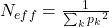 . This is the number of peaks of the same strength that would give the same concentration, so higher values imply a more uniform distribution of amplitudes. Finally, spectral entropy is
 (in nats; calculated over at most 15 retained peaks). A higher value of entropy implies the amplitude is more spread out among the retained peaks. The three measures are averaged across frames to obtain one value per track. I also do a counterfactual amplitude-equalization test. I retain the observed frequency locations in each frame but replace all retained peak amplitudes by
where n is the number of retained peaks. This keeps total retained-peak energy unchanged but equalizes the strengths of all peaks. Then I recompute level-normalized roughness at the same frequency locations, but with the original frame RMS value. If the minor-rougher difference increases, it implies that the original amplitude distribution offsets the effect of frequency placement.
I discuss three versions of the separation profile. The count profile contains the number of frequency pairs that fall into each bin. In addition, the amplitude-weighted profile includes pair strength by summing min(Ai, Aj) over each bin. The roughness-weighted profile uses the full roughness calculation of Sethares in each bin. I compare these profiles to see how much mode information comes from frequency distribution, amplitude intensity, and the overall roughness model. I also do the analysis with different definitions of bins and better representations of separations. In the synthetic triads this major/minor roughness contrast remains in the presence of all these harmonic components; in real music, however, with the 15 largest spectral peaks, this contrast is almost non-existent. Thus, the number of components is not the only factor determining if the roughness relationship survives. The order of those frequencies may also matter.
I first test this in the real recordings. In the 3,000-track progressive sample at N = 15, I ask whether the relationship between mode and roughness changes with harmonic organization. I estimate
where Rnorm is total roughness divided by RMS level, using the 15 strongest spectral peaks. Mode is the continuous major-minor score defined above, with larger values representing more major-like structure. The measure of organization is the harmonic ratio, which is the fraction of the signal’s energy that is assigned to sustained harmonics versus percussive content. The interaction term tests whether the relationship between mode and roughness is different across harmonic organization. As a descriptive comparison, I also divide tracks into lower, middle, and upper thirds of harmonic ratio and compare the major–minor roughness relationship across these groups.
I then run a synthetic experiment to see if harmonic organization helps to preserve the major–minor roughness contrast as spectral complexity increases. I begin with the fundamental frequencies of the root, third, and fifth of each major or minor triad and progressively increase the number of spectral components from N = 3 to N = 30 per chord (1 to 10 harmonics per note).
In the harmonically structured case, further elements follow the harmonic series of the chord tones with amplitudes decreasing according to 0.7n−1 with n the harmonic number. In the disorganized condition, further elements are placed at random between 0.5 and 15 times the triad root frequency and given an amplitude of 0.7. I average the results for the disordered state over 50 random realizations. All signals are normalized to the root mean square (RMS).
I run a 2 x 2 factorial experiment in which I vary the frequency organization (harmonic series vs. random arrangement) and the amplitude distribution (decreasing as 0.7n−1 vs. uniform). The random placement conditions use the same protocol for generating frequencies and average the results over 50 trials. The design assesses the effect of frequency organization and amplitude distribution, independently and jointly, on the major–minor roughness contrast.
I then ask if the interaction-separation profile reveals information about happy and sad expressions in the 1311 happy-sad tracks with ISP data. I evaluate models on activity features (RMS level, spectral flux, onset rate, tempo), tonal features (harmonic ratio, spectral flatness) and mode score taking into account the interaction profile and its three manifestations. Cross-validation folds are grouped by artist.
Prediction and Statistical Inference
Classification models were based on L2-regularized logistic regression (C=1.0, standardized predictors) implemented in scikit-learn35. I apply artist-grouped 5-fold cross-validation to analyze the mode profiles of 9,244 mode-quartile tracks. Happy–sad analyses follow the same procedure on the 1,311 tracks that belong to the mode-quartile sample and have complete interaction spectrum profile (ISP) data, from 2,376 tracks tagged exclusively “happy” or “sad.” Grouping by artist avoids having tracks from the same artist in both the training and test sets of any fold. Classification performance is measured by the area under the ROC curve (AUC), and ∆AUC measures the improvement from adding a set of features. Uncertainty in ∆AUC is assessed using 2,000 paired artist-level bootstrap resamples of the out-of-fold predictions, with the same resampled artists used for both models in each comparison. Confidence intervals for individual AUC values use 2,000 track-level bootstrap resamples of the out-of-fold predictions. Confidence intervals for Cohen’s d use 2,000 artist-level bootstrap resamples. Because of the large sample sizes, I focus on effect sizes and confidence intervals rather than p-values, since even very small effects can be statistically significant.
I report group differences as the standardized mean difference (Cohen’s d), with positive values indicating larger values in minor-like tracks. Thus, a positive roughness difference corresponds to the expected minor-rougher direction. For total roughness, I also employ two one-sided tests (TOST) with a pre-specified equivalence range of |d| < 0.10. This tests whether the major-minor difference is small enough to be practically negligible, not just statistically different from zero. The happy–sad boundary analysis includes four ∆AUC comparisons: adding ISP without and with mode, and adding mode without and with ISP (Supplement Table S5). I adjust the four resulting p-values using the Holm procedure to control the family-wise error rate.
Results
From Simple Sounds to Complex Music
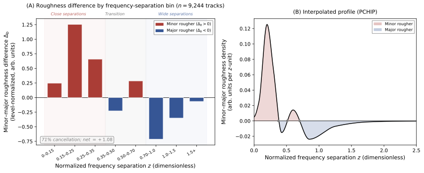
Panel A of Figure 1 shows the Sethares pairwise roughness curve for two pure tones. The minor third, with frequency ratio 6:5 = 1.20, lies above the major third, with ratio 5:4 = 1.25. At a 262 Hz base, the model assigns 40.5% more roughness to the minor third.
The same order is obtained for harmonically complex musical chords. Panel B compares synthetic major and minor triads with each note having harmonic overtones. Averaged over 12 root notes, minor triads are 3.7% rougher than major triads under minimum-amplitude weighting and 5.8% rougher under product weighting. Although it is much smaller than the pure-tone difference, the minor-rougher result survives the addition of harmonic complexity. It is robust to changes in register, tuning system, harmonic decay, and number of harmonics. I also provide views of the synthetic benchmark, such as time-domain waveforms and a continuous frequency-ratio roughness landscape (Supplement Figure S1).
This difference is essentially absent in real polyphonic music. Across 18,486 tracks, continuous mode score is nearly uncorrelated with level-normalized roughness (r = −0.01, p = 0.052). Strongly major-like and minor-like tracks have nearly identical total roughness (d = +0.03, 95% CI [−0.04, +0.09]), with equivalence supported within the prespecified small-effect range |d| < 0.10 (TOST, p < 0.05). I obtain the same result when using product weighting (d ≈ +0.02; equivalence p < 0.01). Thus, a relationship that is pronounced for isolated intervals and remains detectable in synthetic harmonic chords is nearly absent in real recordings.
A similar analysis (Supplement Section S8) based on 30 auditory filters, spaced evenly on the ERB scale39,40, and weighted by energy at their centroid frequencies, also reveals a difference in mode-quartile roughness close to zero (d = +0.01, 95% CI [−0.09, +0.11]).
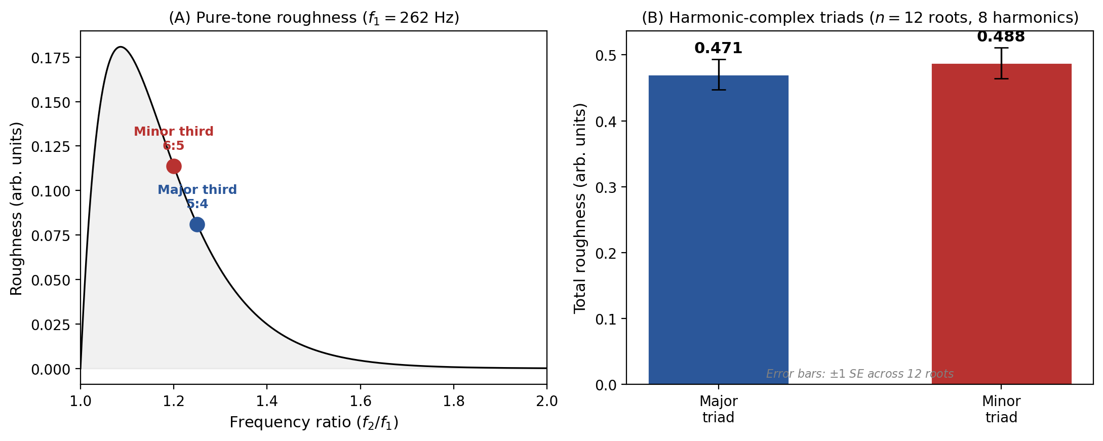
To understand why this difference disappears, I recompute roughness in 3,000 real tracks while increasing the number of dominant spectral peaks from N = 2 to N = 15 (Figure 2). With only the two strongest peaks, minor-like tracks are rougher (d = +0.21). The effect decreases monotonically as more peaks are included in the calculation. The effect is already below the pre-specified small-effect reference |d| = 0.10 at around five to six peaks.
The across-track correlation between retained-peak spectral entropy and level-normalized roughness is -0.02 at N = 2 and +0.32 when N = 15. Thus, as the mode-group difference weakens, roughness becomes more associated with spectral amplitude distribution (Supplement Table S1).
Mode-Related Spectral Structure
The major-minor roughness difference becomes very small as more spectral components are included in the calculation, but this does not tell us whether the difference disappears over the whole spectrum, or whether opposing contributions cancel.
To differentiate between these possibilities, I decompose level-normalized roughness across the eight frequency-separation ranges defined in the Methods, using the 9,244 tracks in the mode-quartile sample. For each separation bin b, define
where Rb is the roughness contributed by frequency pairs in that bin. Positive values of ∆b indicate greater roughness in minor-like tracks, while negative values imply greater roughness in major-like tracks.
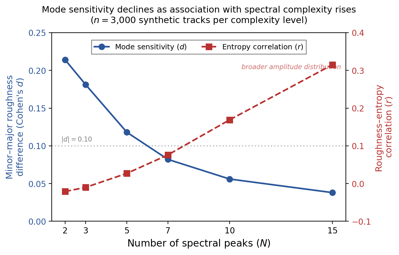
Figure 3A shows the eight bin-specific differences. The pattern is not one of uniform dilution. At close frequency separations, the differences are positive, indicating greater roughness in minor-like tracks. The largest minor excess is at z ∈ [0.15, 0.25), where ∆b = +1.25. At wider separations, the sign reverses in several bins, indicating greater roughness in major-like tracks. For example, ∆b = −0.71 for z ∈ [0.70, 1.0).
The contributions have opposite signs, so when they are added there is largely a cancelation in magnitude. If I add up the absolute difference in all eight bins, it is 3.80. If I add up the signed differences, it is only +1.08. I summarize this cancellation as
Using the underlying bin values, I obtain C = 0.71 (95% bootstrap confidence interval [0.25, 0.99]; 10,000 resamples at the artist level). When the inputs are combined into one overall roughness measure, this eliminates about 71% of the large major-minor difference at particular separation ranges. The eight bins are exhaustive and mutually exclusive, so that the signed group disparities sum exactly to yield the overall group difference using the same averaging procedure: each track is averaged over frames with at least two preserved peaks (see Methods). This methodology drops 0.8% of frames in a 500-track evaluation. The mean track-level difference between this method and the overall frame average of the base extractor is less than 1%.
The bin-wise deviations are plotted as a piecewise cubic Hermite interpolating polynomial (PCHIP) curve in Figure 3B. The curve shows a number of sign changes, reflecting the non-monotonic trend seen above in Panel A: bins 0-2 are positive, bin 3 negative, bin 4 positive, and bins 5-7 negative. Frequency pairs at close separations tend to contribute greater roughness in minor-like recordings, while pairs at wider separations tend to contribute greater roughness in major-like recordings. But there is no clear crossover. I also observe the same opposite sign pattern when combining the eight bins into four, three or two larger bins, with a cancelation rate of 61-71%. The small overall change in frequency separations conceals a large structure, and does not signal any systematic breakdown of the major-minor relation.
If aggregation cancels out structure related to mode, keeping the locations of roughness over frequency separations might preserve information missed in the sum. In line with this prediction, adding the eight-bin interaction-separation profile to a model that already includes peak harmonicity, total roughness, and spectral amplitude-distribution metrics improves classification of mode-quartile groups by ∆AUC = +0.055 (p < 0.001, see Supplement Table S2). This improvement is robust to alternative binning schemes and smooth representations of separation (Supplement Table S4). Therefore, data hidden by aggregation is partially recovered by preserving the frequency-separation structure of the original pairwise inputs. The decomposition shows that the immediate source of the near-zero total is cancellation between opposing contributions across separation ranges.
Frequency Arrangement and Spectral Amplitude Distribution
I separate out two reasons for the overall roughness difference: the number of frequency pairs that can contribute and the amplitude strength of those pairs. As defined in the Methods section, active pairs are retained-peak pairs with z < 1.5. Minor-like recordings contain slightly more active pairs per frame than major-like recordings (21.9 vs. 21.0; d = +0.21; Table 1). This excess is concentrated toward the closer frequency-separation ranges, including ranges that receive relatively high weight from the Sethares roughness kernel. The frequency arrangement of the spectral components thus tends to support the anticipated minor-rougher correlation.
The average active-pair amplitude weight,  /RMS, is lower in minor-like than in major-like tracks (66.1 vs. 70.7;
 =
 0.25), an effect comparable in magnitude to the pair-count difference. The amplitude-weight difference thus cancels most of the minor-like advantage in the number and distribution of active pairs, resulting in a total active roughness,
 /RMS, that is only slightly larger in minor-like tracks (d = +0.03).
| Quantity | Minor | Major | Ratio | d |
| Active pairs per frame (Nactive) | 21.9 | 21.0 | 1.044 | +0.21 |
| Mean pair amplitude (W̄active/RMS) | 66.1 | 70.7 | 0.935 | −0.25 |
| Active roughness (Ractive /RMS) | 100.4 | 99.2 | 1.012 | +0.03 |
Why is the typical major-like pair more strongly weighted? The amplitude-distribution measures defined in the Methods suggest a common explanation. Major-like tracks have a lower top-3 amplitude share (0.539 vs. 0.553), a larger effective number of peaks (Neff = 7.81 vs. 7.51), and higher spectral entropy. These differences suggest a somewhat more even distribution of amplitude across the dominant spectral peaks of major-like tracks.
This is important because the basic Sethares specification gives weights to each pair based on min(Ai, Aj). When the spectral amplitude is concentrated on a few dominant peaks, many pairs have at least one weak component and their impact on roughness is limited. The less dominant member of a standard pair is stronger when the amplitude is more evenly distributed, giving rise to a larger pairwise amplitude weight.
The observed difference in mean pairwise amplitude weight under the min(Ai, Aj) criterion (d = −0.25) is in line with these amplitude-distribution variations: major-like tracks distribute amplitude more uniformly, implying that the weaker component of a standard pair is comparatively stronger. Because both the amplitude-distribution metrics and the pair strength are derived from the same spectral amplitudes, the association is descriptive evidence. As an associational decomposition, Table S6 shows that including the three amplitude-distribution metrics reduces the mode coefficient by 70%.
The preceding evidence within the model suggests that frequency arrangement tends to favor minor-like tracks, while amplitude organization offsets part of this advantage. I explicitly test this mechanism in the roughness calculation by normalizing the retained-peak amplitudes, preserving their observed frequency locations and the total retained-peak energy. Within each frame, all retained amplitudes are replaced by
and level-normalized roughness is then recomputed using the same frequency structure and the original frame RMS.
If amplitude differences partly offset the minor-rougher tendency associated with frequency arrangement, equalizing amplitudes should make that difference larger. Panel A of Figure 4 shows that minor-like tracks have more roughness-relevant frequency pairs, while Panel B shows that major-like tracks have more evenly distributed amplitudes. Panel C shows the differences in roughness for separation ranges before and after amplitude equalization. For the observed amplitudes minor-like tracks are rougher in four bins and major-like tracks in the other four. After equalization, minor-like tracks are rougher in all eight bins.
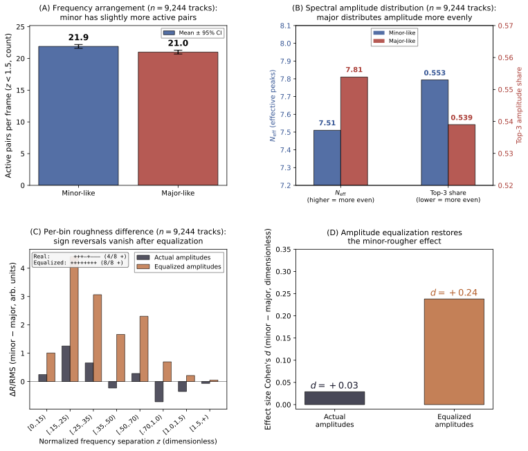
Panel D shows the effect of these changes on total roughness. Given the observed amplitudes, the difference between minor-like and major-like is small (d = +0.03, 95% CI [−0.04, +0.09]). After within-model amplitude equalization, it increases to d = +0.24 (95% CI [+0.17, +0.30]). In this comparison the frequency locations do not change. Thus the larger minor-rougher effect appears after removing amplitude differences. The observed amplitude distribution makes up for much of the difference in frequency arrangement in the model.
The results are similar when I use the alternative product weighting, w = A1A2. The minor-like minus major-like difference in mean pair amplitude weight is slightly smaller in magnitude (d = −0.20). The aggregate active-roughness difference remains near zero (d = +0.02), with 75% cancellation. Equalizing amplitudes increases the minor-rougher difference to d = +0.23, and minor-like tracks are again rougher in all eight bins. Both weighting schemes produce the same pattern of cancellation.
Finally, I ask how much of the mode information in the separation profile is due to frequency-pair locations alone. I compare three profiles, separated into eight separation bins. The count profile counts the number of pairs in each bin. Pair amplitudes also are included in the amplitude-weighted profile. The full Sethares calculation is used for the roughness-weighted profile.
I first add each profile to a baseline containing harmonicity and total roughness, but excluding the amplitude-distribution features used in Table S2. The count profile achieves an AUC improvement of +0.076, compared to +0.067 for the amplitude-weighted profile and +0.060 for the roughness-weighted profile (Supplement Table S3). Combining count and roughness profiles together brought AUC to 0.637 (95% CI [0.618, 0.656]) from 0.555 (95% CI [0.539, 0.575]), the highest estimate of all models in Table S3. The increase is +0.082 (95% CI [+0.051, +0.101]).
I then compare the profiles without the baseline covariates. AUC is improved by +0.029 when combining the count and roughness profiles compared to the roughness profile alone, and by +0.023 compared to the count profile alone (both p < 0.001). These results suggest that much of the mode information in the roughness profile is already present in the arrangement of frequency pairs. The two profiles overlap, but each has information that is not available in the other: pair counts alone help distinguish the mode groups, while the roughness-weighted profile adds information in addition to those counts.
Harmonic Organization Is Associated with Preservation of the Signal
The above analysis shows that the amplitude distribution can offset the minor-rougher tendencies due to the frequency arrangement. But why does this tendency appear to be stronger for some complex spectra than others? The overall difference for real recordings is almost zero while for synthetic triads there is a small rougher-difference even with many harmonic partials. Thus, part of the result may be due to the number of components. How those components are arranged may also matter.
I study this question in real recordings using the interaction regression in Eq (2). For the 3000-track progressive sample, with K = 15 retained peaks, I regress level-normalized roughness on continuous mode score, harmonic ratio and their interaction. The dependent variable is RMS-normalized roughness, which is not standardized in the regression. Both predictors are standardized to have mean zero and unit variance, and their product forms the interaction term. All standard errors and confidence intervals are based on HC1 heteroskedasticity-robust estimates.
The coefficients are  = 0.3 (SE = 0.7, 95% CI [1.6, +1.0], and
 = 0.66) for mode score and
 = 12.2 (SE = 0.9, 95% CI [13.9, 10.5], and
 0.001) for harmonic ratio. The interaction coefficient is negative (
 = 1.9, SE = 0.8, 95% CI [3.5, 0.3], and = 0.02). Since higher mode scores imply more major-like structure, this negative interaction means that the fitted mode-score slope becomes more negative when harmonic ratio increases. In other words, the predicted minor-like minus major-like roughness difference becomes more positive as harmonic organization increases. The negative interaction is also observed in the full mood-tagged subset (
 = 18,486; = 0.8, 95% CI [1.5, 0.2], = 0.015). This analysis includes the original 3,000 tracks and thus provides a sample-expansion check.
The same trend is also observed when tracks are sorted by the level of organization. In the most organized third, minor-like versus major-like roughness has a positive difference (d = +0.06). In the least organized third, the difference reverses (d = −0.12). As such, the contrast is more positive in the case of recordings with a stronger tonal organization.
I then test the role of frequency arrangement in synthetic chords. Starting with the root, third, and fifth of major and minor triads, I increase the number of spectral components from N = 3 to N = 30 per chord. When added frequencies follow the chord’s harmonic structure, the minor-minus-major roughness difference is +4.63% at N = 15 and stays above +2% through N = 30. When nonfundamental frequencies are instead placed randomly, with the same component count and equalized overall RMS level, the difference falls to +0.92% at N = 15 and becomes indistinguishable from zero at N ≥ 20. Averaged across amplitude conditions, harmonic rather than random frequency placement increases the percentage minor–major roughness difference by approximately 5 percentage points. Averaged across frequency conditions, decaying rather than uniform amplitudes increase it by approximately 2.7 percentage points. With either amplitude schedule, minor chords are still rougher when frequencies follow a harmonic structure. Random placement flips the sign for both schedules. The amplitude distribution changes the size of the difference, but does not explain the minor-rougher difference in the harmonic spectra by itself.
Adding components does not necessarily eliminate the minor-rougher relationship. In these tests, the difference is better preserved when frequencies are in a harmonic structure. Along with the results on amplitude equalization, this provides a reason for not attributing total roughness solely to the number of components: the arrangement of frequencies and the distribution of amplitudes are also important.
Exploratory Happy–Sad Analysis
In an investigative analysis I question whether the interaction-separation profile may also be used to predict the happy-sad labels given by uploaders. The analysis uses 1,311 tracks with complete interaction-separation profile data and uploader-supplied happy–sad labels. The AUC increased by +0.011 (raw p = 0.042; Holm-adjusted p = 0.084) when the profile was added to a model with activity-related acoustic characteristics and tonal-organization metrics. This improvement is not statistically significant after correction. The increase is reduced to +0.002 (raw p = 0.330; adjusted p = 0.330) when the mode score is added to the baseline. Further predictive information is provided by the mode score. It increases the AUC by +0.046 over the Activity + Harm baseline and +0.036 when the interaction-separation profile is already included (both p < 0.001; Supplement Table S5).
Thus, the profile is useful for telling major-like from minor-like recordings, but adds little to the prediction of happiness vs. sadness given the mode score. I do not see any statistically significant improvement after adjusting for these factors. The findings here are an indication of how the recordings were tagged by the uploaders, not what the listeners hear or how the recordings make them feel.
Discussion
In the Sethares model, major-like and minor-like recordings have almost the same total roughness, but their contributions vary over frequency-separation ranges. Minor-like recordings have slightly more roughness-relevant frequency pairs. But the amplitudes of the dominant peaks in major-like recordings are more evenly distributed, so the typical pair carries more weight with the primary minimum-amplitude weighting. These differences act in opposite directions on roughness, and when summed much of the difference across separation bins is canceled. I find the same pattern for product weighting.
Thus a small difference in total roughness does not imply similarity in the underlying spectra. The frequency-pair arrangement is useful in separating the mode-quartile groups aside from total roughness and peak harmonicity. The harmonic-organization analyses also indicate that the change in the minor-rougher difference cannot be explained solely by the addition of components. In the synthetic experiments, the difference is better preserved when the components have a harmonic structure. Amplitude distribution also changes the size of the difference.
The exploratory happy–sad analysis provides weaker evidence of a connection to emotion labels. The interaction-separation profile results in a small estimated gain in predicting uploader-supplied tags, and this gain is not statistically significant when mode score and other acoustic features are included. These tags do not directly measure listeners’ perceptions or their emotional responses. The results do not show roughness to be responsible for the well-known association between musical mode and emotion41,42.
There are a number of constraints (Supplement S8). The mode score is an indicator of the acoustics, not a verified classification. Some of the correlation between mode score and roughness is likely because both are derived from the same spectra. The recordings also differ in ways that this analysis may not fully capture. The genre, instrumentation and production techniques could cause the differences between major-like and minor-like compositions. The collection is predominantly Western43. Stratified and mixed-effects analyses44 further reveal that a small overall correlation remains after controlling for genre, instrumentation and artist composition. Adding genre covariates lowers the mode coefficient by about 9.5%. These tests investigate some possible explanations, but others may remain.
Frequency arrangement and amplitude distribution are not fully separate in this analysis: amplitude determines which peaks are retained. Equalization changes the amplitudes of those selected peaks while keeping their frequencies fixed. It tests how the model responds to that change; it does not isolate independent causal mechanisms or measure a perceptual response. Equalization raises the estimated group difference from d = +0.03 to d = +0.24. This shows that amplitude distribution affects the model’s output, but the resulting standardized effect is still small and does not establish an audible or practically important difference. Future work should compare the mode score with independent annotations, test equalization through acoustic resynthesis and controlled listening experiments, and examine whether the findings hold across roughness models27,8.
Conclusion
The small difference in total roughness hides larger differences across frequency-separation ranges that largely cancel within the Sethares model. Minor-like recordings have more roughness-relevant pairs, but the amplitude distribution in major-like recordings gives individual pairs greater weight. Equalizing peak amplitudes makes the minor-rougher difference larger. This difference also persists more clearly when frequencies remain harmonically organized. These results explain how the model arrives at a small total difference, but not what causes the spectral differences in recordings or whether listeners perceive them.
Code Availability
The code is available from the author upon request.
Supplementary Material
References
- S. Dalla Bella, I. Peretz, L. Rousseau, N. Gosselin. A developmental study of the affective value of tempo and mode in music. Cognition. Vol. 80, pg. B1–B10, 2001, https://doi.org/10.1016/S0010-0277(00)00136-0. [↩] [↩]
- T. Fritz, S. Jentschke, N. Gosselin, D. Sammler, I. Peretz, R. Turner, A. D. Friederici, S. Koelsch. Universal recognition of three basic emotions in music. Current Biology. Vol. 19, pg. 573–576, 2009, https://doi.org/10.1016/j.cub.2009.02.058. [↩]
- H. von Helmholtz. On the sensations of tone as a physiological basis for the theory of music. Longmans, Green, and Co., 1875. Translated by A. J. Ellis from the 3rd German edition (original work published 1863). [↩] [↩]
- R. Plomp, W. J. M. Levelt. Tonal consonance and critical bandwidth. Journal of the Acoustical Society of America. Vol. 38, pg. 548–560, 1965, https://doi.org/10.1121/1.1909741. [↩] [↩] [↩]
- L. H. Arnal, A. Flinker, A. Kleinschmidt, A.-L. Giraud, D. Poeppel. Human screams occupy a privileged niche in the communication soundscape. Current Biology. Vol. 25, pg. 2051–2056, 2015, https://doi.org/10.1016/j.cub.2015.06.043. [↩]
- L. H. Arnal, A. Kleinschmidt, L. Spinelli, A.-L. Giraud, P. Megevand. The rough sound of salience enhances aversion through neural synchronisation. Nature Communications. Vol. 10, pg. 3671, 2019, https://doi.org/10.1038/s41467-019-11626-7. [↩]
- W. A. Sethares. Tuning, timbre, spectrum, scale, 2nd ed. Springer, 2005, https://doi.org/10.1007/b138848. [↩] [↩] [↩]
- P. N. Vassilakis. Auditory roughness as a means of musical expression. Selected Reports in Ethnomusicology. Vol. 12, pg. 119–144, 2005. [↩] [↩] [↩]
- T. Popescu, M. P. Neuser, M. Neuwirth, F. Bravo, W. Mende, O. Boneh, F. C. Moss, M. Rohrmeier. The pleasantness of sensory dissonance is mediated by musical style and expertise. Scientific Reports. Vol. 9, pg. 1070, 2019, https://doi.org/10.1038/s41598-018-35873-8. [↩]
- F. Stolzenburg. Harmony perception by periodicity detection. Journal of Mathematics and Music. Vol. 9, pg. 215–238, 2015, https://doi.org/10.1080/17459737.2015.1033024. [↩]
- E. Terhardt. Pitch, consonance, and harmony. Journal of the Acoustical Society of America. Vol. 55, pg. 1061–1069, 1974, https://doi.org/10.1121/1.1914648. [↩] [↩] [↩]
- T. Eerola, I. Lahdelma. The anatomy of consonance/dissonance: evaluating acoustic and cultural predictors across multiple datasets with chords. Music & Science. Vol. 4, pg. 20592043211030471, 2021, https://doi.org/10.1177/20592043211030471. [↩]
- J. H. McDermott, A. J. Lehr, A. J. Oxenham. Individual differences reveal the basis of consonance. Current Biology. Vol. 20, pg. 1035–1041, 2010, https://doi.org/10.1016/j.cub.2010.04.019. [↩]
- R. Parncutt, G. Hair. Consonance and dissonance in music theory and psychology: disentangling dissonant dichotomies. Journal of Interdisciplinary Music Studies. Vol. 5, pg. 119–166, 2011. [↩]
- T. Eerola, I. Lahdelma. Register impacts perceptual consonance through roughness and sharpness. Psychonomic Bulletin & Review. Vol. 29, pg. 800–808, 2022, https://doi.org/10.3758/s13423-021-02033-5. [↩]
- I. Lahdelma, T. Eerola. Single chords convey distinct emotional qualities to both naïve and expert listeners. Psychology of Music. Vol. 44, pg. 37–54, 2016, https://doi.org/10.1177/0305735614552006. [↩]
- I. Lahdelma, T. Eerola. Cultural familiarity and musical expertise impact the pleasantness of consonance/dissonance but not its perceived tension. Scientific Reports. Vol. 10, pg. 8693, 2020, https://doi.org/10.1038/s41598-020-65615-8. [↩]
- D. L. Bowling, K. Gill, J. D. Choi, J. Prinz, D. Purves. Major and minor music compared to excited and subdued speech. Journal of the Acoustical Society of America. Vol. 127, pg. 491–503, 2010, https://doi.org/10.1121/1.3268504. [↩]
- D. L. Bowling, J. Sundararajan, S. Han, D. Purves. Expression of emotion in Eastern and Western music mirrors vocalization. PLoS ONE. Vol. 7, pg. e31942, 2012, https://doi.org/10.1371/journal.pone.0031942. [↩]
- G. Carraturo, V. Pando-Naude, M. Costa, P. Vuust, L. Bonetti, E. Brattico. The major-minor mode dichotomy in music perception. Physics of Life Reviews. Vol. 52, pg. 80–106, 2025, https://doi.org/10.1016/j.plrev.2024.11.017. [↩]
- D. L. Bowling, D. Purves. A biological rationale for musical consonance. Proceedings of the National Academy of Sciences. Vol. 112, pg. 11155–11160, 2015, https://doi.org/10.1073/pnas.1505768112. [↩]
- P. M. C. Harrison, M. T. Pearce. Simultaneous consonance in music perception and composition. Psychological Review. Vol. 127, pg. 216–244, 2020, https://doi.org/10.1037/rev0000169. [↩]
- T. Eerola, A. Friberg, R. Bresin. Emotional expression in music: contribution, linearity, and additivity of primary musical cues. Frontiers in Psychology. Vol. 4, pg. 487, 2013, https://doi.org/10.3389/fpsyg.2013.00487. [↩]
- L. Gagnon, I. Peretz. Mode and tempo relative contributions to “happy-sad” judgements in equitone melodies. Cognition and Emotion. Vol. 17, pg. 25–40, 2003, https://doi.org/10.1080/02699930302279. [↩]
- J. C. Hailstone, R. Omar, S. M. D. Henley, C. Frost, M. G. Kenward, J. D. Warren. It’s not what you play, it’s how you play it: timbre affects perception of emotion in music. Quarterly Journal of Experimental Psychology. Vol. 62, pg. 2141–2155, 2009, https://doi.org/10.1080/17470210902765957. [↩]
- R. Parncutt. Harmony: a psychoacoustical approach. Springer-Verlag, 1989, https://doi.org/10.1007/978-3-642-74831-8. [↩] [↩]
- P. Daniel, R. Weber. Psychoacoustical roughness: implementation of an optimized model. Acta Acustica united with Acustica. Vol. 83, pg. 113–123, 1997. [↩] [↩]
- G. M. Bidelman, A. Krishnan. Neural correlates of consonance, dissonance, and the hierarchy of musical pitch in the human brainstem. The Journal of Neuroscience. Vol. 29, pg. 13165–13171, 2009, https://doi.org/10.1523/JNEUROSCI.3900-09.2009. [↩]
- M. Cousineau, J. H. McDermott, I. Peretz. The basis of musical consonance as revealed by congenital amusia. Proceedings of the National Academy of Sciences. Vol. 109, pg. 19858–19863, 2012, https://doi.org/10.1073/pnas.1207989109. [↩]
- D. A. Schwartz, C. Q. Howe, D. Purves. The statistical structure of human speech sounds predicts musical universals. The Journal of Neuroscience. Vol. 23, pg. 7160–7168, 2003, https://doi.org/10.1523/JNEUROSCI.23-18-07160.2003. [↩]
- D. Bogdanov, M. Won, P. Tovstogan, A. Porter, X. Serra. The MTG-Jamendo dataset for automatic music tagging. In Machine Learning for Music Discovery Workshop, ICML, 2019. [↩]
- A. Aljanaki, Y.-H. Yang, M. Soleymani. Developing a benchmark for emotional analysis of music. PLoS ONE. Vol. 12, pg. e0173392, 2017, https://doi.org/10.1371/journal.pone.0173392. [↩]
- M. Zentner, D. Grandjean, K. R. Scherer. Emotions evoked by the sound of music: characterization, classification, and measurement. Emotion. Vol. 8, pg. 494–521, 2008, https://doi.org/10.1037/1528-3542.8.4.494. [↩]
- B. McFee, C. Raffel, D. Liang, D. P. W. Ellis, M. McVicar, E. Battenberg, O. Nieto. librosa: audio and music signal analysis in Python. In Proceedings of the 14th Python in Science Conference, pg. 18–24, 2015, https://doi.org/10.25080/Majora-7b98e3ed-003. [↩]
- F. Pedregosa, G. Varoquaux, A. Gramfort, V. Michel, B. Thirion, O. Grisel, M. Blondel, P. Prettenhofer, R. Weiss, V. Dubourg, J. Vanderplas, A. Passos, D. Cournapeau, M. Brucher, M. Perrot, E. Duchesnay. Scikit-learn: machine learning in Python. Journal of Machine Learning Research. Vol. 12, pg. 2825–2830, 2011. [↩] [↩]
- C. L. Krumhansl. Cognitive foundations of musical pitch. Oxford University Press, 1990, https://doi.org/10.1093/acprof:oso/9780195148367.001.0001. [↩]
- D. Temperley. Music and probability. MIT Press, 2007. [↩]
- B. J. Aarden. Dynamic melodic expectancy. PhD dissertation, Ohio State University, 2003. [↩]
- B. R. Glasberg, B. C. J. Moore. Derivation of auditory filter shapes from notched-noise data. Hearing Research. Vol. 47, pg. 103–138, 1990, https://doi.org/10.1016/0378-5955(90)90170-T. [↩]
- B. C. J. Moore, B. R. Glasberg. Suggested formulae for calculating auditory-filter bandwidths and excitation patterns. Journal of the Acoustical Society of America. Vol. 74, pg. 750–753, 1983, https://doi.org/10.1121/1.389861. [↩]
- P. N. Juslin, D. Västfjäll. Emotional responses to music: the need to consider underlying mechanisms. Behavioral and Brain Sciences. Vol. 31, pg. 559–575, 2008, https://doi.org/10.1017/S0140525X08005293. [↩]
- P. N. Juslin. From everyday emotions to aesthetic emotions: towards a unified theory of musical emotions. Physics of Life Reviews. Vol. 10, pg. 235–266, 2013, https://doi.org/10.1016/j.plrev.2013.05.008. [↩]
- J. H. McDermott, A. F. Schultz, E. A. Undurraga, R. A. Godoy. Indifference to dissonance in native Amazonians reveals cultural variation in music perception. Nature. Vol. 535, pg. 547–550, 2016, https://doi.org/10.1038/nature18635. [↩]
- R. H. Baayen, D. J. Davidson, D. M. Bates. Mixed-effects modeling with crossed random effects for subjects and items. Journal of Memory and Language. Vol. 59, pg. 390–412, 2008, https://doi.org/10.1016/j.jml.2007.12.005. [↩]