Evaluating Atmospheric Influences on Star Count and Visibility in Commercial Telescope Imaging

Abstract

Modern-day astrophysics has a heavy dependency on observations of stellar sources, as these detections provide key insights into how various stellar populations and their structures have evolved over time. Over the last few decades, the quality of ground-based observations has improved drastically; however, most assessments of astrophotography still rely heavily on visual judgements of the image, which make the quality subjective. Metrics such as “sharpness” or “clarity” obscure the depth of any quality discussion of the image. This study develops and applies a reproducible and quantitative pipeline that brings professional-style validation methods to consumer-grade telescope data such as that from the ZWO SeeStar S50, through catalogue cross-matching against Gaia and a formal photometric check of the flux–magnitude relationship, hence substituting a subjective evaluation with an objective one. The pipeline detects stellar sources in FITS images using the DAOStarFinder algorithm and validates them against the Gaia catalogue through the World Coordinate System transformation available in the FITS metadata. Detection parameters were optimised per file using a plateau-stability criterion. This yielded a median FWHM of 5.5 pixels (range 3.6–6.5), a detection threshold of 2.5σ, and a Gaia magnitude limit of G ≤ 20, from the set of 17 files with sufficient bright matched sources. Across these files, the photometric slope between Gaia G magnitude and log DAO flux came out to be −2.266 ± 0.537, a value that is consistent with the theoretical value of −2.5 (one-sample t-test, t(16) = 1.80, p = 0.091), confirming the pipeline’s photometric validity. In addition, we created a normalised detection ratio in the form (matched/catalogue) stars at Gaia G magnitude less than 14; this ratio ranged from 0.00 to 0.59 across the 18 observations, with a mean of 0.26. This ratio is correlated against atmospheric variables derived from the Copernicus ERA5 dataset. Only one of the proxies used (the seeing proxy) produced a correlation of the correct sign (r = −0.522; R² = 0.27; p = 0.026). Three out of five variables were seen to have changed signs, and after application of a Bonferroni correction for the number of comparisons made, only one variable (low-level cloud cover) remained significant; this had a physically unrealistic trend and would therefore be explained by a density effect due to the field being crowded. Henceforth, the analysis of atmospheric variables in this study is reported as relatively exploratory and underpowered. Nevertheless, the pipeline still contributes as a strong and reproducible quantitative validation workflow for consumer-grade astrophotography. The robust atmospheric characterisation will still require a much larger dataset and homogeneous target selection over extended periods, with multivariate confounder control systems.

Keywords: Light pollution, Astronomical photometry, CCD photometry, Star counts, Atmospheric seeing, Sky surveys

Introduction

A key aspect of modern-day astrophysics is the observation of various stellar sources, these sources provide us with valuable insights into structure and evolution of star populations. Hubble’s (1929) discovery of a linear relation between the distances of extra-galactic nebulae and their radial velocities demonstrated the importance of linking observable properties of celestial bodies to their physical characteristics¹. Over the following decades, the way astronomy is perceived has shifted from purely observational to data driven models and methods, which help us create precise and reproducible measurements of stellar distributions².

The development of standardized data formats such as the Flexible Image Transport System (FITS) have been crucial to the transformation of this field, data formats such as the FITS can store image data and important metadata, values such as the exposure time, instrument configuration, and celestial coordinates^3,4,5. These meta values are extremely crucial for calibrating and mapping out celestial coordinates. Alongside this, the development of open source computational tools have further accelerated the growth, the Astropy library for instance provides frameworks for FITS manipulation and coordinate transformations^6,7. The major role of Astropy was in particular, the extraction of the World Coordinate System (WCS), this enables us to convert pixel coordinates into sky coordinates, which allowed us to make direct comparisons between the pixel level detections and map them directly out onto the sky through catalogues⁸.

Star catalogues, including the Gaia Star Catalogue represent a major advancement in data driven astronomy. The Gaia mission has produced high-precision astrometric and photometric data for over a billion stars, generating a detailed three-dimensional map of the Milky Way^9,10,11,12. The Gaia star Catalogue’s accuracy becomes an important aspect as it is the reference through which validation for observational data occurs by confirming those sources.

Alongside the growth of catalogues and computational tools, the development of automated detection algorithms have been crucial. Beyond DAOStarFinder, source-extraction tools such as SExtractor are also widely used¹³. One of the most widely used methods is the DAOStarFinder (hereafter also abbreviated DAO), originally derived from the DAOPHOT algorithm, developed and introduced by Peter Stetson¹⁴. The detections found through the algorithm are done by identifying local maxima that agree upon an expected point spread function (PSF)¹⁵, which in turn allows us to filter out the background noise from real star detections¹⁶. DAO-based detections have been extensively used for both professional and amateur astronomical studies¹⁷. One key factor to note is that the accuracy of detections from DAO is heavily reliant on the certain parameters, such as the full width at half maximum (FWHM) and background noise estimations, these parameters must be tuned based on the observational conditions¹⁸.

Although methods and technology has improved for better ground-based observations, the whole process is still limited by environmental factors, particularly light pollution, increased artificial and environmental brightness lowers the visibility of faint stars and lowers signal to noise ratio during imaging^{19,20,21,22,23,24}. Studies worldwide demonstrate this effect by using atmospheric models to show the widespread impact of artificial illumination on night sky visibility, especially in urban regions. Other models, for instance the ones developed by Garstang, further explain how scattered light contributes to skyglow and degrades observational quality^22,23.

Finally, atmospheric conditions cause discrepancies in the variability of the number of stars detected. Parameters such as relative humidity, wind speed, cloud cover, and low cloud cover directly influence atmospheric transparency and stability. Increased humidity and aerosol levels scatter and absorb incoming starlight, which reduces the signal strength and lowers the detection completeness. Wind speed is used as a proxy for atmospheric turbulence (seeing), where unstable air can cause images to distort and broaden the point spread function, which in turn will overall reduce the detection accuracy, transparency proxies derived from atmospheric data indicate the clarity of the sky, with lower transparency corresponding to greater extinction of stellar flux. Additionally, cloud cover is another important environmental indicator, wherein low-cloud cover impacts the incoming light by obstructing its path and creating attenuation across the image. In conclusion, these factors affect the signal to noise ratio as well as the reliability of source detection, making them extremely crucial in observational astronomy.

This investigation accounts for these effects by making the comparison of the number of normalised stars detected throughout the image with various atmospheric conditions. Star counts from FITS data are correlated with variables such as humidity, wind speed, cloud cover, and derived seeing and transparency proxies, and validated against Gaia catalogue data. Through which we are able to better understand the influence of atmospheric conditions on accuracy and completeness of detections.

Motivation

Most professional astronomers assess astrophotographic images using one of two approaches: a qualitative (subjective) approach or a quantitative one. Astrophotographers often describe the quality of their photographs using terms such as “quality,” “definition,” or “sharpness,” based on the observer’s personal opinion or the observations made at the time. Almost all professional astronomical observations, by contrast, are validated by objective measures, including detecting objects against catalogues, using statistical methods to identify objects within images, and documenting observing conditions. A significant methodological gap exists between these two types of observational practice: very few student or low-budget astronomy projects, which typically use relatively low-quality instruments, undergo validation procedures similar to those used in professional astronomy — including cross-matching detections against trusted catalogues, systematically optimising parameters through data analysis, and validating detected features using formal photometry. To bridge this methodological gap and provide a degree of scientific validity to images obtained from accessible instruments, this research establishes an entirely quantitative assessment procedure for consumer-grade astrophotography. Beyond establishing a quantitative evaluation process, there is also a need to integrate additional context into the determination of image quality: image quality is affected not only by the instrumentation but also by environmental factors such as atmospheric conditions and sky conditions (including moon phase, cloud cover, and sky brightness). The author’s long-term observations of decreasing night-sky visibility due to increasing urbanisation provided the impetus to document these environmental changes objectively rather than subjectively. On the other hand formal and professional astronomy relies strongly on validation by the detection of objects: Detected sources are cross-matched against trusted astrometric catalogues, detection algorithms are tuned using statistical metrics, and observing conditions are carefully documented.

Therefore, currently a gap between professional methods and commonplace workflows (small-telescope or student-led astrophotography projects) exist. This gap limits the scientific strength and interpretability of data captured from accessible instruments. The motivation behind this project is to bridge this gap, the goal will be accomplished by developing a fully functional and quantitative pipeline that has the ability to evaluate astrophotography data, which is the fundamental principle used in my professional settings. The overarching goal is to shift the evaluation of astrophotography from qualitative analysis to a quantitative measure.

Additionally, this work supports the idea of the need for contextual data integration for astrophotography. It is important to note that images are not only influenced by the type of telescope or detector, but atmospheric conditions play a crucial role in the output of data, such as sky brightness, cloud cover, and moonlight. These projects are often not accounted for in small-scale projects.

This work is intended to benefit student researchers who require scientifically defensible methodologies for image analysis, citizen-science initiatives in which data quality varies widely and needs objective validation, amateur astronomers seeking to understand why certain nights or setups yield better results, and educational programs aiming to teach authentic, data-driven astronomy rather than purely visual techniques.

Background information

FITS files

In the context of our project the FITS files form the foundational input for all the subsequent star-detection and validation analyses. Since the foundation of this project relies on the detections of stars through DAOStarFinder and Gaia’s astrometric catalogue, the preservation of each pixel is essential for complete observation, and hence exemplifying the importance of metadata stored in the fits file. The flexible image transport system (FITS) file consists of the standard archival and data for interchange of format to astronomical data. This has remained as the principal method/medium for scientific imaging since its adoption by NASA in the late 1970s. A FITS file is not designed solely to act as a medium of image conversion, but instead it is a rigorously structured scientific dataset, capable of encoding instrument behaviour, observational conditions, and calibrated pixel intensities with complete reproducibility with merely the METADATA. The formation of the FITS file is based on one or more Header/Data units (HDU’S). THe header is composed of 80-character ASCII keywords, values ,component cards, documents and all relevant metadata: telescope and detector identifiers, exposure parameters, gain, readout noise, sensor temperature, Julian date, observatory coordinates, atmospheric conditions, and any processing history. This metadata ensures that the image is scientifically interpretable independent of the original acquisition environment.

The data unit in the FITS file stores the pixel array in an uncompressed, linear format (Usually 16 or 32 bit integers, or floating point decimal values), hence preserving the complete dynamic range of the detectors and meta data, allowing for rigorous and accurate photometric and astrometric data analysis. Unlike consumer image formats, such as JPEG or JPG– FITS data files preserve data in its original state, maintaining absolute integrity in the astronomical signals captured. Such data conservation is absolutely indispensable for quantitative tasks, such as plate solving, flat fielding, bias subtraction, cosmic-ray ejection and photometric analysis.

World Coordinate System

Within the scope of our project, the world coordinate system bridges the gap between algorithmic star detection in image space and physical validation of celestial coordinates. The World Coordinate System (WCS) is the data that relates image-plane pixel coordinates directly to the absolute celestial coordinates on the sphere. WCS is embedded directly within the FITS file, inside the headers, through a series of standardized keywords, WCS enables an astronomical image to be interpreted as a metrically accurate projection of the specific area/region in the sky rather than a simple two-dimensional intensity array. The WCS specification defines the reference world coordinates (CRVAL1, CRVAL2 headers), the corresponding reference pixel (CRPIX1, CRPIX2), the linear transformation matrix (CDij or PCij), and the adopted celestial projection (e.g., gnomonic/TAN, orthographic/SIN, or AITOFF). Collectively, these parameters describe the local astrometric solution, including plate scale, rotation, parity, and, where applicable, distortion corrections.

Accurate WCS information is often obtained through processes such as astrometric plate solving²⁵, wherein detected star centroids in the image are matched against positions from an external astrometric catalogue (e.g., Gaia DR3). The solved WCS results in the best fitting transformation that aligns the image to an absolute celestial reference frame with extreme precision. The resulting WCS mapping facilitates a wide range of scientific operations: precise astrometric measurement, field identification, multi-epoch registration, photometric cross-matching, and spatial modelling of sky-brightness distributions.

Tools and apparatus used

All the images were captured using the ZWO SeeStar S50, a telescope optimized for wide field astronomical imaging²⁶. The technical specifications of the telescope include a 50 mm apochromatic triplet refractor with a 250 mm focal length (f/5), this allows the telescope to capture the image with low-aberration, fast optics suitable for short exposure and sky brightness measurements. Imaging is performed with a Sony IMX462 CMOS sensor (1920 × 1080, 2.9 μm pixels), offering high sensitivity, low read noise, and strong performance under light-polluted conditions. The device records data in 16-bit FITS format, retaining all metadata necessary for photometric and astrometric analysis.

The telescope is mounted on a motorized alt-azimuth Go-To system with automated tracking. Although alt-az mounts experience field rotation over long integrations, the S50’s rapid stacked imaging workflow minimizes this limitation for environmental sky assessments. Its internal plate-solving module provides accurate World Coordinate System (WCS) solutions for each FITS file, enabling pixel-level mapping to RA/DEC coordinates and ensuring consistent comparisons across observing sites. Integrated dual-band Hα/OIII filters suppress broadband sky-glow, improving contrast for star detection and background measurement. The system’s automated focusing, exposure control, and mobile-based operation make it a reliable, field-deployable platform for reproducible light-pollution mapping.

Processing data on Python

All the data processing and analysis throughout this project was completely conducted using Python due to its extensive ecosystem of astronomical libraries and its suitability for reproducing scientific workflows. The FITS files were fed through a standard I/O routine, which works to preserve both the pixel data arrays and all the header metadata. Preprocessing steps include background estimations for the sky, noise characterisation, and normalization, which are important to standardise detections through images with varying sky-brightness and exposure conditions. Background levels were estimated using robust statistical methods to reduce the influence of bright sources, while noise properties were inferred directly from the image statistics to ensure physically meaningful detection thresholds.

Astrometric data was accessed directly through the headers stored in the FITS files, allowing us to utilize pixel-to-sky transformation of data from data in the FITS through the embedded WCS solution. Detected sources, their position and other useful data were stored in structured arrays, this allowed us to efficiently filter, cross-match and variable sweep (such as FWHM, DAO thresholds). This pipeline built with python was designed to operate modularly, which allowed us to apply the same analysis across different files. This process ensured reproducibility, minimized subjective bias in parameter selection, and allowed systematic exploration of how detection performance varies with image conditions.

DAOStarFinder

Stellar sources were detected through the DAOStarFinder algorithm, which identifies point-like sources by locating local maxima that match an expected point spread function (PSF). The DAOStarFinder algorithm works completely in the pixel space, by modelling stars as approximately Gaussian profiles characterized by a specified full width at half maximum (FWHM). This parameter represents the spatial extent of a stellar image and is influenced heavily by atmospheric conditions, optical performance, and tracking stability. Selecting an appropriate FWHM is henceforth crucial, values that are too small suppress real stars, while excessively large values increase false detections by merging light noise structures together as one and background fluctuations.

DAOStarFinder evaluates candidate detections by convolving the image with a Gaussian kernel and applying a significance threshold relative to the background noise. Therefore this threshold works as a barrier, allowing only sources exceeding this threshold and satisfying shape constraints (set by the FWHM) as retained as real detections. Additionally this algorithm returns centroid coordinates, peak intensity, and profile statistics, which form the basis for subsequent astrometric and photometric validation. Throughout the process of this project, the DAOStarFinder algorithm was used iteratively across a controlled range of FWHM and threshold values which allowed us to find the most optimum combinations of values outputting strong detections. This approach allowed detection performed to be quantitatively assessed and chosen rather than arbitrarily detecting stellar bodies.

Gaia query

The detections made by DAOStarFinder are often accurate in identifying real astrophysical objects, but we need an extra layer of confirmation and validation, hence an external astrometric reference catalogue was required. To fulfill this need we used the extensive catalogue provided by Gaia queries, which provides high-precision positions for over a billion stars. The catalogue queries were performed systematically within python, using sky coordinates of the centroids derived from the FITS files. For each image, a region-based query was executed to retrieve all Gaia sources within the field of view, ensuring complete coverage for cross-matching.

The process of cross-matching was performed by comparing the celestial coordinates of DAO detections with Gaia positions using a fixed angular match radius. Star matches within this radius were classified as true detections, while unmatched sources were treated as false positives and hence eliminated. By repeating this procedure across varying DAOStarFinder parameters (FWHM and threshold), the relationship between detection sensitivity and astrometric reliability could be quantitatively evaluated in terms of the matched stars. Importantly, this process allowed the optimal FWHM to be identified not by maximizing raw detection counts, but by maximizing agreement with Gaia while minimizing false-positive matches.

Methodology

Step 1: Raw astronomical image acquisition and initial representation

The raw data analysis begins with a pipeline where FITS file data (astronomical data) is directly gathered using a CMOS detector during observational exposure. At this stage, the data is fundamentally a two dimensional grid of pixel intensities, where each pixel encodes the number of photons detected from a small region of the sky during the exposure time. It is important to note that these pixel values are affected by a wide range of factors, which include the astrophysical source (stars in this case), the background sky noise, the instrumental effects including detector noise, readout artifacts, and atmospheric distortions. Additionally, it is important to note that the current data we have is unprocessed, so it does not include anything beyond intensity measurements.

To preserve the scientific integrity of the data, the data is stored in the Flexible Image Transport System, better known as FITS. This file type is effective in story astronomical data as it allows for both the image array and extensive metadata to coexist within a single file. The metadata present in the FITS file include information on the observation time, the configuration of the telescope, and calibration parameters. What is more important is that FITS eschews from compressed and remodelling the data in the file, essentially preserving the original photon statistics without any compromising on initial data. At this point the image can be interpreted as a visual star field, but it remains an unprocessed numerical dataset awaiting systematic extraction of astrophysical information.

Step 2: FITS loading and separation of image data and metadata

The following steps include the development of the pipeline, alongside the data extraction from the FITS files. Once a FITS file is selected for analysis, it is loaded into the pipeline, wherein the image data and the header information are directly extracted as separate entities. The image itself is extracted and stored as a NumPy array, where we are able to directly view the intensities of each and every pixel, while the header is parsed into a structured metadata object. This step is extremely crucial, because throughout the later stages of the analysis, the image itself and the headers are used for disparate parts of the analysis. The image is used for detections, centroiding and photometric analysis, while the header provides the contextual information required to interpret the image in a physical and celestial framework.

The pipeline that was made at this stage did not have the ability to transform or filter any of the data. The goal to this stage was to preserve the image exactly as recorded while ensuring it is accessible for subsequent processing. Additionally, one crucial role that the headers play is that they contain World Coordinate System (WCS), these are parameters and coordinated that describe how a certain pixel located in the image is positioned when mapped out onto the sky, but these are not yet applied. The image remains entirely in pixel space, meaning that any detected feature is defined only by its location within the detector grid, not by its right ascension or declination.

Step 3: Channel handling and grayscale image preparation

Astronomical images can be stored as a single channel intensity map or a multi-channel image which is obtained from stacking multiple single-channel maps, resulting in a color combined intensity map, with certain RGB values for each pixel. However, most star detection algorithms, such as DAOStarFinder can only take two-dimensional intensity distributions as input. Hence, whenever a multi-channel image is encountered in the pipeline, it converts them into a grayscale representation by averaging across channels. This operation preserves the total signal while reducing channel-specific noise fluctuations and eliminating color dependence, which is irrelevant for positional detection.

It is important to note that the sole purpose for the grayscale image is analytical only. The original multi-channel image is still preserved throughout this process for visualization and presentation of the authentic image. This separation allows the detection decisions to be made on analytical and numerical criteria, while the visual outputs are faithful to their original capture. The grayscale image is efficient to isolate the brightness structure of the field, allowing the detection algorithm to focus only on identifying significant light intensity peaks. By removing the factor of color complexity at this stage, the pipeline ensures that the following detections are independent of visual color artifacts, reinforcing the objectivity and reproducibility of the detection process for other such FITS files.

Step 4: DAOStarFinder run

Following all the necessary steps performed earlier, the source detection algorithm of DAOStarFinder, from the Photoutils package, was run on the globular cluster M71 (Messier 71). As mentioned earlier, the FITS file was altered dimensionally, where the multi-channel data was converted to a two-dimensional grayscale intensity map via channel averaging. This ensured that the data was fully preserved, while making the file compatible with the algorithm.

Before applying the detection algorithm to the image, we estimated the background noise characteristics using sigma-clipped statistics. Particularly, the mean and standard deviation of the background was computed after excluding outlier pixel values, this ensured that we eliminate the influence of bright stars and cosmic artifacts which emit rays. Then the detection threshold was defined as a multiple of the background standard deviation, which in this case was around ∼5σ, this ensured that only statistically intense peaks of noise were considered as a real detection.

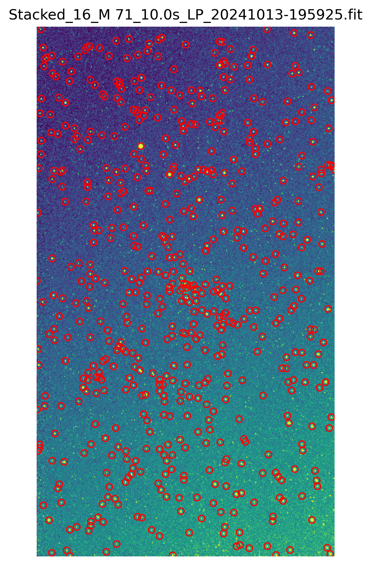
After all the above steps were considered, we then ran the DAOStarFinder algorithm, this algorithm models stellar profiles using a two-dimensional Gaussian approximation of the point spread function (PSF), considering a Full Width at Half Maximum (FWHM) parameter tuned to match the expected seeing conditions of the observation, based on the clipped statistics considered and calculated earlier. The algorithm then finds intensity peaks that match the set parameters and conditions, and detects them as identified sources (The sources in the Figure 1 are marked by a red outline, each red outline is one real detection of the algorithm).

Step 5: Small radius Gaia search

To validate and evaluate the reliability of the DAOStarFinder detection, a precautionary step was implemented, in which we compared the output from the DAOStarfinder algorithm with an external astronomical catalogue, which in this case was Gaia. Through the use of the World Coordinate System (WCS), already embedded within the FITS file, we were able to convert the pixel space into celestial coordinates (RA/DEC). A cone search, with a relatively small radius, was performed on the Gaia database with a defined angular radius corresponding to a selected region of the image.

This query to the Gaia catalogue then returned the number of stars (N_Gaia) that are expected to truly exist within the specific region, this was set a baseline for the “true” detections, the output from the DAOStarFinder algorithm run providing us with detected stars based on intensity thresholds and point spread function characteristics, yielding the number of detected sources (N_DAO) within the same radius.

To check for the reliability of our DAO detection, a detection fraction was computed as: 

This ratio revealed how complete and effective the algorithm is at finding true stellar sources, while values closer to 1 would indicate a high detection accuracy, lover values will indicate missed detections or limitations in the setup due to noise, thresholding or environmental constraints.

Step 6: Large radius Gaia search

To further validate the small radius Gaia search, a larger detection was ran on the entire field of the image. Unlike the small-radius validation, which samples a localized region, this approach ensures that the entire observational field is represented, providing a more concrete assessment of detection completeness. Similar to the small radius search the central pixel coordinates of the image were transformed into celestial coordinates (right ascension and declination), the cone was defined by the angular separation between the centre of the image and one of the image corners. By doing this, the entire rectangular image was covered. Furthermore, the row limit was asynchronously removed (ROW_LIMIT = -1), which allowed us to retrieve data on every single star present in that observational field.

Step 7: Plotting stars back onto the image

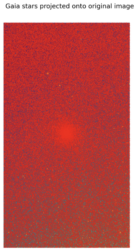
To further validate the spatial consistency between detected and catalogued sources, the Gaia dataset was projected back onto the original FITS image using the World Coordinate System (WCS) transformation. Each Gaia source, defined by its celestial coordinates (right ascension and declination), was converted into pixel coordinates using the inverse WCS mapping. This allowed direct overlay of catalogue stars onto the observational image plane as seen in Figure 2.

The resulting visualization plots Gaia sources as markers across the full image, enabling a qualitative assessment of positional alignment and source density. As observed, the overlay produces a high-density distribution of points, particularly concentrated toward the core of the globular cluster M71. This reflects both the intrinsic stellar density of the cluster and the depth of the Gaia catalogue, which includes faint sources that may not be detectable in the observational data.

This step is critical in identifying systematic discrepancies between catalogue data and algorithmic detections. Regions where Gaia sources are present but DAOStarFinder fails to detect stars indicate limitations due to noise thresholds, crowding effects, or insufficient resolution. Conversely, detected sources without Gaia counterparts may indicate false positives or transient artifacts.

Step 8: Optimising the PSF through FWHM parameter sweep

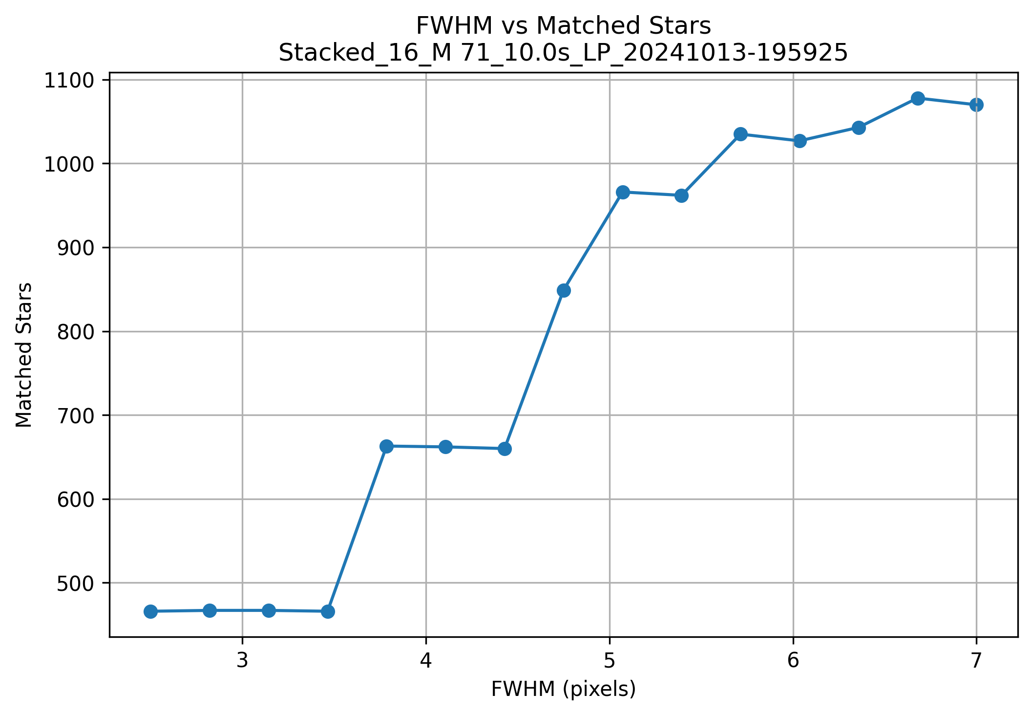
To define the most optimal point spread function (PSF) width for the detections, a sweep for an extensive range of the Full Width at Half Maximum (FWHM) was conducted. The FWHM value in the DAO function directly influences the algorithm’s sensitivity to stellar sources.

A range of FWHM values from 2.5 to 7.0 pixels was sampled at regular intervals. For each FWHM value, DAOStarFinder was applied to the background-subtracted image, where the background level was estimated using sigma-clipped statistics and removed via median subtraction. The detection threshold was fixed at 7σ above the background noise to ensure consistency across all trials. Detected sources were then cross-matched with Gaia catalogue stars (filtered to G ≤ 16) using a positional tolerance of 2 pixels, producing a relationship between FWHM and matched star count, as observed in Figure 3.

Instead of selecting the value of FWHM that outputs the maximum number of stars, a stability based approach was used instead. The curve demonstrating the relationship between matched stars and FWHM values was smoothed using a Gaussian filter, and its numerical gradient with respect to FWHM was computed. Parts of the graph where the gradient approached zero were identified as plateau regions, indicating that detection performance is insensitive to small variations in FWHM.

The optimal FWHM was selected as the midpoint of the longest contiguous plateau  The plateau for the FWHM sweep was determined quantitatively. A plateau was defined as a window of at least four consecutive FWHM samples whose average matched-star count was greater than or equal to 90% of the highest matched-star count across the full FWHM sweep. From this group, the leftmost (lowest-value) qualifying window was used as the representative window, and the optimum FWHM value was extracted from it., ensuring that the chosen value reflects a stable and physically representative approximation of the point spread function, rather than being influenced by local maxima or noise-induced fluctuations.

Step 9: DAO vs Gaia

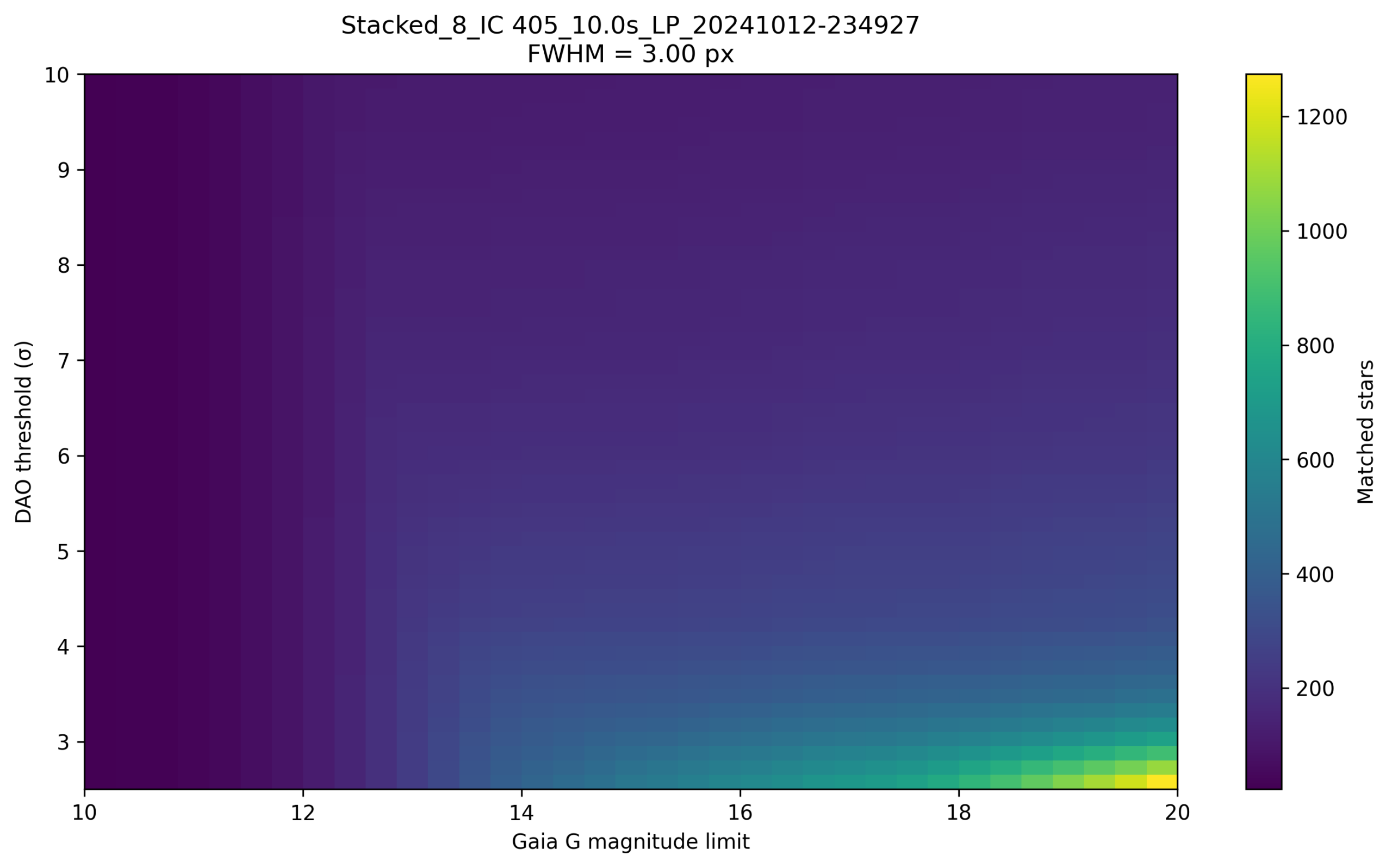
Next we refined the detection process to further strengthen our detection process, a simultaneous, two parameter sweep was conducted based on the DAOStarFinder detection threshold and the Gaia catalogue magnitude limit. For this detection process the FWHM was fixed at 3 as determined from prior FWHM optimization. The detection threshold for DAOStarFinder was varied between 2.5σ and 10σ above the sigma-clipped background standard deviation, while the Gaia catalogue was filtered across magnitude limits from G = 10 to G = 20.

For each possible combination of parameters, the DAOStarFinder was applied to the background subtracted image, and then were subsequently cross matched within a tolerance range/match radius of 2 pixels The 2-pixel tolerance was selected from a dedicated match-radius sweep (0.5–5.0 pixels in 30 steps), choosing the plateau where the matched-star count became insensitive to radius (gradient below 0.05). Its false-match rate can be estimated as N_DAO × πr² × ρ_Gaia, where ρ_Gaia is the catalogue source density per pixel over the 1080 × 1920 image; for the bright-star metric used in the analysis (G < 14) this yields negligible contamination (of order 1% of matched sources even in the densest fields), whereas at the full catalogue depth (G ≤ 20) chance coincidences become substantial in crowded fields, which further motivates the G < 14 restriction. The radius also exceeds the sub-pixel astrometric residuals of the plate-solved WCS solutions, so genuine matches are not excluded.. The number of matched stars was recorded, producing a two-dimensional dataset representing detection performance across parameter space, as observed in Figure 4.

Step 10: Gaia vs DAO optimal values

After this sweep’s data was collected and stored, the next goal was to find the optimal DAO detection threshold and Gaia magnitude limit were systematically determined for each FITS image using a plateau-based analysis. For The optimisation of parameters is partly two-dimensional: the detection threshold and the Gaia magnitude limit are varied jointly over an entire grid, so the effects of and interactions between both variables are captured simultaneously. The full width at half maximum (FWHM), by contrast, is optimised separately in a prior sweep at a fixed 7σ threshold, rather than optimising all parameters over a full three-dimensional grid. Because the FWHM optimum is defined by the location of a plateau — a region insensitive to slight parameter variation — rather than by a sharp peak, and because changing the detection threshold produces only minor shifts in the location of that plateau, no systematic bias is expected from the sequential approach. A full three-dimensional grid search would nonetheless represent a more rigorous validation, and is noted as an additional step for future work. each sweep output, the data results were transformed into a two-dimensional parameter surface of matched star counts as a function of detection threshold and magnitude limit. After which the gradient of the surface was calculated along both the axes, and zones with a lower gradient (stable zones) were identified as plateau zones  For the two-dimensional threshold–magnitude surface, plateau cells were identified as those on the matched-star surface whose normalised gradient magnitude was less than or equal to 0.10 and whose matched-star count was at least 80% of the surface maximum. Where no cell satisfied both criteria, relaxed thresholds were used: cells with a normalised gradient magnitude at or below 0.15 and a matched-star count of at least 75% of the peak were treated as plateaus; otherwise the surface peak was taken as a default. The cross-matching radius itself was determined using a sweep from 0.5 to 5.0 pixels in 30 steps, selecting the plateau where the gradient of matched count with respect to radius was smallest (below 0.05).. These zones represent stable parameter combinations of Gaia and DAO where detection performance is not affected by small variations.

Step 11: Matched stars data collection

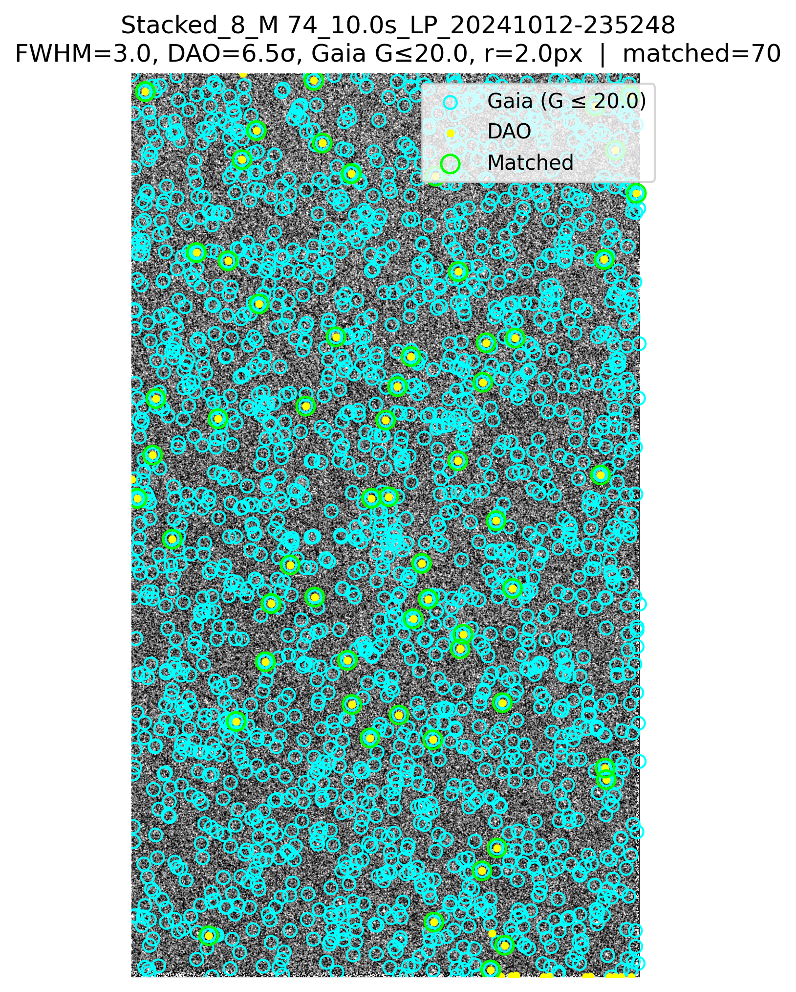
After collecting data from the sweeps and identifying optimal threshold and limits from the plateau analysis for FWHM, Gaia limit and DAO threshold, a final cross-matching procedure was performed to construct the most optimal number of stellar source detections for each image. Gaia catalogue data were first loaded and transformed from celestial coordinates (right ascension and declination) into pixel coordinates using the World Coordinate System (WCS). Sources falling outside the image boundaries were excluded, and a magnitude filter was applied to ensure consistency with the observational detection limit.

Next DAOStarFinder was applied to the background image using the optimised detection thresholds, which give us the centroid positions and flux measurements for all detected sources. A nearest-neighbour matching algorithm, implemented through a k-dimensional tree (cKDTree), was used to efficiently associate each Gaia source with the closest DAO detection within the predefined matching radius. The stellar sources identified by DAO that overlaid with confirmations for Gaia sources were then plotted back onto the original image for visual representation of the matches, as observed in Figure 5.

Step 12: Photometric validation of matched sources

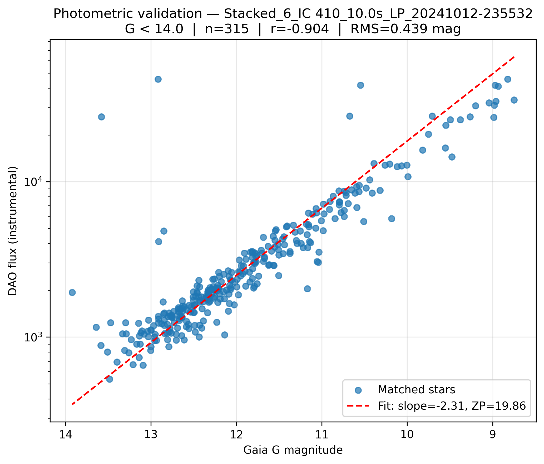
To further validate the consistency of the matched dataset from the previous analysis, an additional step was taken. A photometric validation step was performed, this validation step checked the Gaia magnitude of each individual stellar source and compared it with the instrumental flux values obtained from the DAOStarFinder. The Gaia G-band magnitude for each star was compared with the logarithm of its corresponding DAO flux value, and hence outputted a purely logarithmic relationship between the two variables, as observed in Figure 6.

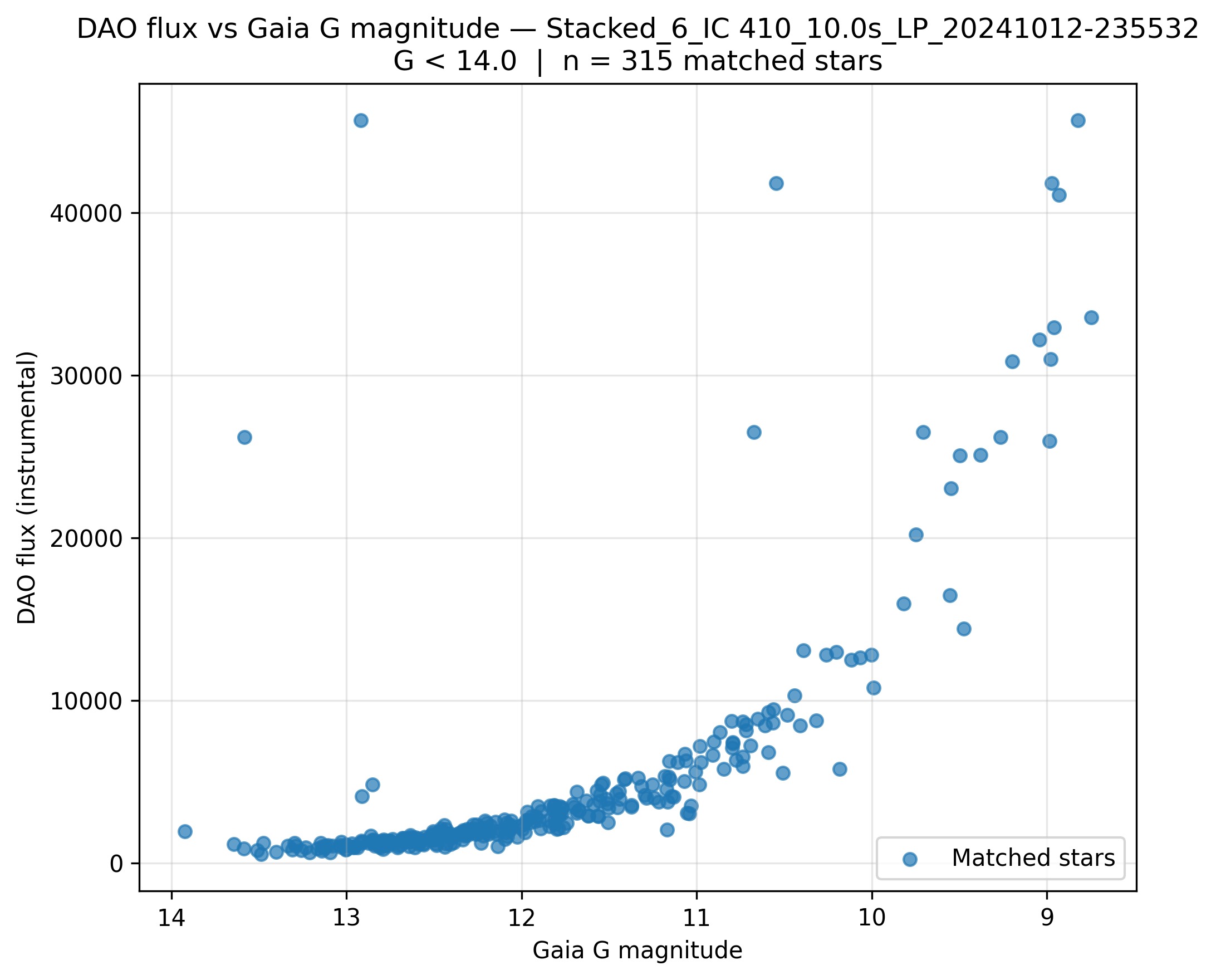
A scatter plot was generated for each dataset, with Gaia magnitude on the x-axis (inverted to reflect increasing brightness) and DAO flux on a logarithmic scale on the y-axis. A strong negative correlation is expected, as brighter stars (lower magnitudes) should correspond to higher detected flux values. Additionally the very same data was plotted on a non-logarithmic DAO scale against the same magnitude, this resulted in an expected exponential trend, since these variables are logarithmic to each other in nature, as observed in Figure 7.

Step 13: Pixel-level validation of source detection

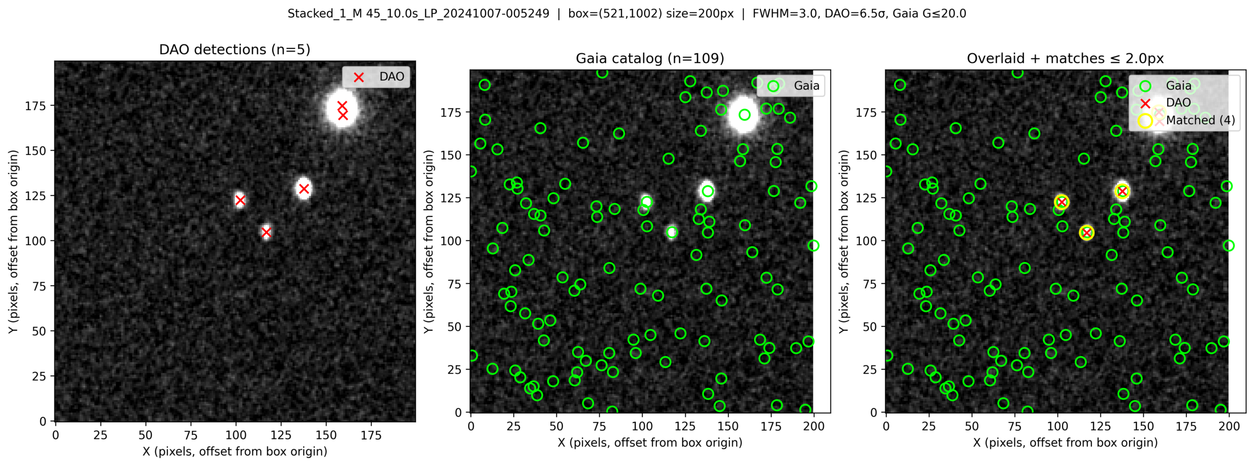
The next step of verification of the matched stars is to check the spatial accuracy of the detection algorithm, is through a localised validation performed on the sub-region of the image. A 200 × 200 pixel box was extracted, centred on the median position of Gaia sources to ensure an accurate representation of the stellar field. Next, DAO was applied to this given 200 × 200 region using the optimised variables.

Meanwhile, simultaneously Gaia catalogue stars were filtered to only include stars within that 200 × 200 region and were projected back onto the pixel coordinated using the WCS transformation function, through which we were able to create a visualisations of an overlay where DAO detections and Gaia sources were projected onto the sub-image, enabling qualitative comparison of positional alignment.

Using a K-dimensional tree, each DAO detection was matched to the closest Gaia source within a tolerance of 1 pixel. Finally the number of successful matches were recorded, this helped us define a direct measure of sub-pixel accuracy, as observed in Figure 8.

Step 14: Extraction of atmospheric data from ERA5 and analysis

The next step processed in the pipeline was the extraction of atmospheric data, this was done to study the impact of environmental conditions on the number of normalised star detections. The data was extracted from the Copernicus ERA5 reanalysis dataset^27,28. This dataset provides globally gridded and time resolved estimates of environmental conditions from satellites and numerical data modelling. For each FITS file, the corresponding data was extracted based on parameters of individual observation time and location. The extraction gave us data points for total cloud cover, low-level cloud cover, relative humidity, and wind speed at 10 m altitude. Additionally, derived proxies for atmospheric seeing and transparency were included to approximate optical observing conditions. This data was then structured corresponding to their respective fits files, which made sure each data point had a corresponding FITS file, allowing us to identify the relationship between these variables and the atmospheric conditions.

To analyse the relationship between atmospheric condition and number of normalised FITS files, scatter plots were generated for each variable with detection efficiency on the y-axis and the atmospheric parameter on the x-axis. Linear regression was applied to analyse trends, with coefficients of determination (R^2) and p-values were calculated to assess the strength and statistical significance of correlations.

Step 15: Estimation of sky brightness and light pollution

To quantify the effect of background sky brightness on detection performance, a photometric calibration procedure was implemented to estimate sky brightness in units of magnitudes per square arcsecond²⁹. For each FITS image, sigma-clipped statistics were used to determine the median background signal, representing the sky contribution per pixel. This value was normalised by exposure time and converted into surface brightness using the pixel scale derived from the WCS solution.

To establish an absolute photometric scale, aperture photometry was performed on stars matched between DAO detections and Gaia catalogue sources. Circular apertures were used to measure stellar flux, while surrounding annuli provided local background estimates. Using Gaia G-band magnitudes and measured fluxes, a photometric zero-point was calculated for each image by taking the median of individual star-based calibrations.

The sky brightness was then computed by applying the zero-point to the background flux, yielding values in mag/arcsec^2. This metric provides a direct measure of light pollution, with lower values indicating brighter (more polluted) skies.

Finally, sky brightness was compared against detection efficiency and source density, enabling analysis of how increasing background illumination impacts the ability to detect stellar sources. When sky brightness was included as a predictor in the correlation analysis alongside the ERA5 variables, it showed no significant relationship with the normalised detection ratio across the 14 files with a valid estimate (r = +0.248, p = 0.393; bootstrap 95% confidence interval [−0.33, +0.73], which includes zero). The absence of the expected negative trend is consistent with the narrow range of sky brightness sampled (14.2–15.6 mag/arcsec²) and with the G < 14 restriction of the metric to bright stars least affected by sky background.

Results and discussion

Photometric confirmation analysis

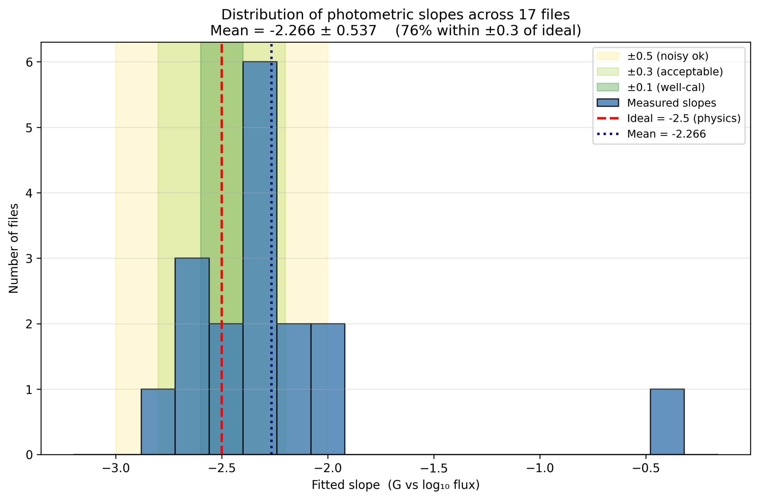
An additional step was carried out to check whether the DAO vs Gaia pipeline was producing real detections rather than capturing random noise, hence through the results from the photometric confirmation step, and a fundamental relationship between DAO flux and Gaia G magnitude, G = -2.5log₁₀(F) + ZP = -2.5log₁₀(F) + ZP, a simple test was ran to check the validity. Since a slope of -2.5 is established and fixed as per the direct relationship, it allows us to use it as a target against which the pipeline can be tested. For all the observations the matched stars above with the G < 14 magnitude were retained, and were plotted against the log₁₀(DAO Flux), and the results from each file were aggregated. The distribution of slopes across the 18 usable observations had a mean of -2.266 ± 0.537, and 76% of files fell within ± 0.3 of the physical ideal and the rest falling within the range of -2.7 to -2.0. To check whether this deviation had any statistical significance, we conducted a one-sample t-test comparing the distribution of fitted slopes against the theoretical slope value of −2.5. Across all files the deviation was not significant (t(16) = 1.80, p = 0.091; 95% confidence interval [−2.54, −1.99], which contains −2.5). This indicates that the mean photometric slope lies within the expected relationship. Excluding the LDN 888 session, whose anomaly is discussed below, the mean slope of the remaining 16 observations was −2.385 ± 0.223 and remained close to the ideal (t(15) = 2.06, p = 0.057). Significance was calculated using a two-sided one-sample t-test comparing the per-file fitted slopes against the −2.5 reference value. Furthermore, a single outlier was identified, with a slope of -0.35 (Stacked_3_LDN 888) reflected that this outlier was not produced due to errors in the pipeline, but rather due to the specific observation session The LDN 888 region contains a large area of dark nebula, so the field is mostly obscured by diffuse extinction rather than being populated with point sources. Only 28 bright stars (G < 14) were identified in the data for the field, compared with 633 catalogued, which results in the lowest detection efficiency in the dataset at 0.044. Given that only a very limited number of photometric points are available to fit a slope, and that many of those points fall within areas of nebulosity that affect the estimated local background and exhibit variability, the slope would be expected to show significant scatter due to small numbers rather than because of any error in the instrument or the pipeline processing. In fact, removing the session file significantly tightened the slope distribution from −2.266 ± 0.537 to −2.385 ± 0.223 while not substantially changing the average; the anomaly is therefore clearly associated with this one session.. This validation step shows us that each detection is physically meaningful and valuable and they have a basis to be analysed for in subsequent atmospheric data analysis, as observed in Figure 9.

Overview of the atmospheric analysis

The relationship between the various atmospheric conditions and the stellar detection was investigated through comparing a normalised matched-star count across all images against the various environmental conditions, derived through the ERA5 reanalysis data. The goal was to see how different conditions have an effect on the detection efficiency in relation to cloud cover, wind speed, seeing, and atmospheric transparency for the 18 observations in the dataset. Detection efficiency was expressed as a normalised ratio to account for the differences between the type of stellar source we captured. Different fields will always contain different numbers of Gaia catalogue stars, for example a crowded field near the galactic plane contains many times more stars than a sparse high-latitude field, hence the raw number of matched detections is not comparable between observations. Therefore, by normalizing the number of catalogued stars present in the field produces a metric that is field size and density independent and is a direct metric for efficiency.

Normalisation and analysis procedure

For each observation, the detection ratio was computed as 

Both the numerator as well as the denominator were restricted to stars that were brighter than Gaia G = 14, this choice for the cut-off was made due to the photometric validation stage of the pipeline, it showed that faint sources (G > 14) are dominated by low signal-to-noise detections and matching noise that scatter away from the expected logarithmic flux-magnitude relationship. Hence restricting the ratio to G < 14 removes faint star noise and ensures that the stars are genuinely detectable on a clean frame. Defined this way, the ratio is a detection efficiency bounded between 0 and 1, with higher values indicating more complete recovery of the catalogue stars present in the field. The denominator was computed using the Gaia catalogue stars within the image using the WCS header, and applying the G < 14. The denominator was computed by projecting Gaia catalogue coordinates into the image coordinate system using the WCS header, counting all catalogue stars falling within the image bounds, and applying the G < 14 cut.

Low-level cloud cover

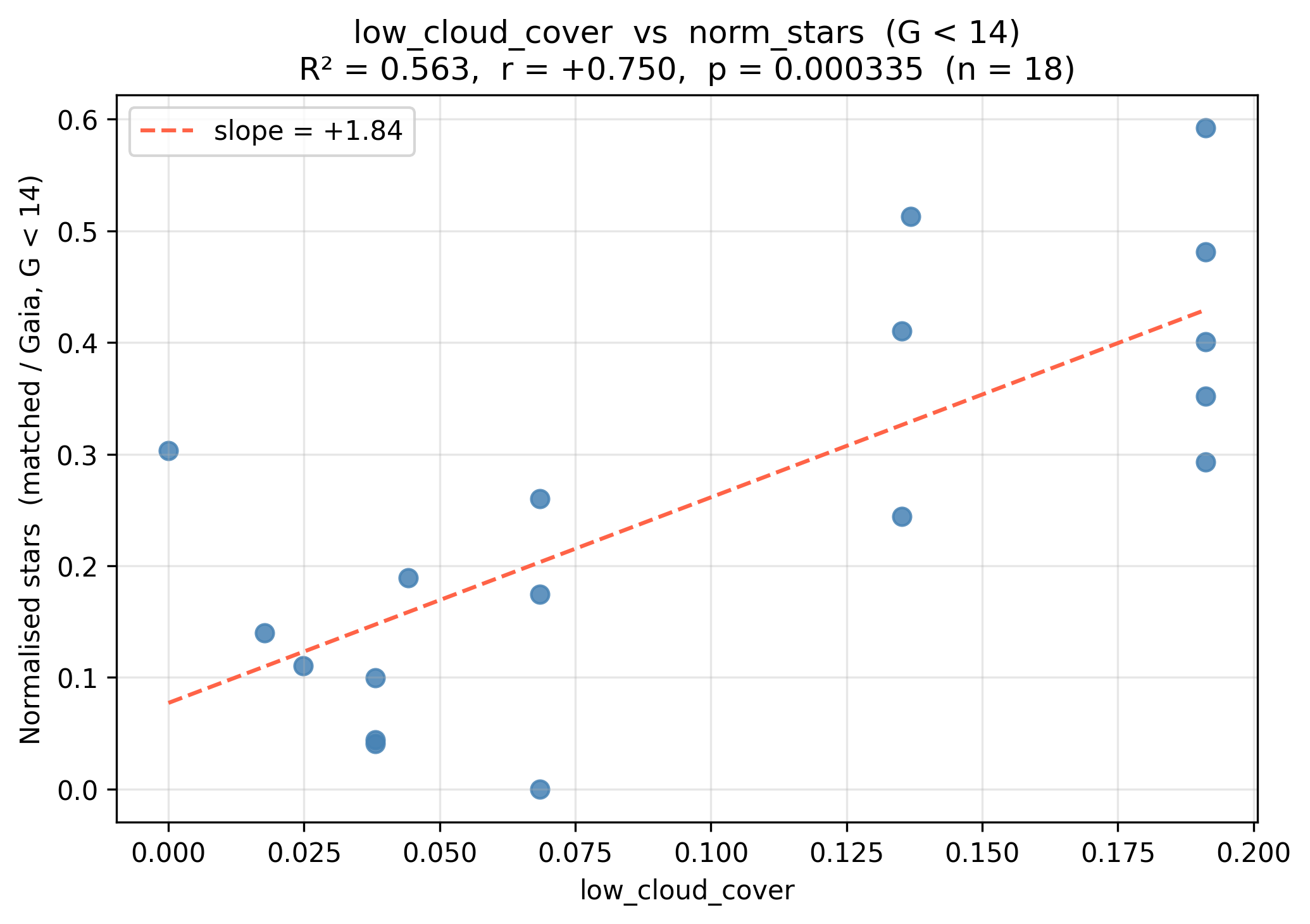
Low level cloud cover had produced positive correlation in the dataset, with with r = +0.750, R^2 = 0.563, p = 3.35 × 10^-4, and slope = +1.84. The correlation is both statistically strong and numerically large. However, scientifically the correlation is supposed to be negative, this discrepancy in the output could be due to a few reasons, such as the observations under higher low-level cloud fractions coincided with higher detection ratios, henceforth the detection does not support the direct interpretation, It should be noted that this interpretation is not attributable to an atmospheric effect. A positive correlation between low-level cloud cover and detection fraction is physically impossible, so it is important to note that it is a confounded artefact. The likely cause of this artefact is field density: across the dataset the detection ratio is negatively related to the number of bright catalogue stars in the field (r = −0.47, p = 0.047 against log field density), because in a high-field-density region the DAOStarFinder algorithm recovers a smaller fraction of the catalogued stars. Nights with low cloud-cover values coincided with sparser fields and produced false, spurious data points. Accordingly, no atmospheric conclusion should be drawn from this analysis. As observed in Figure 10.

Seeing proxy

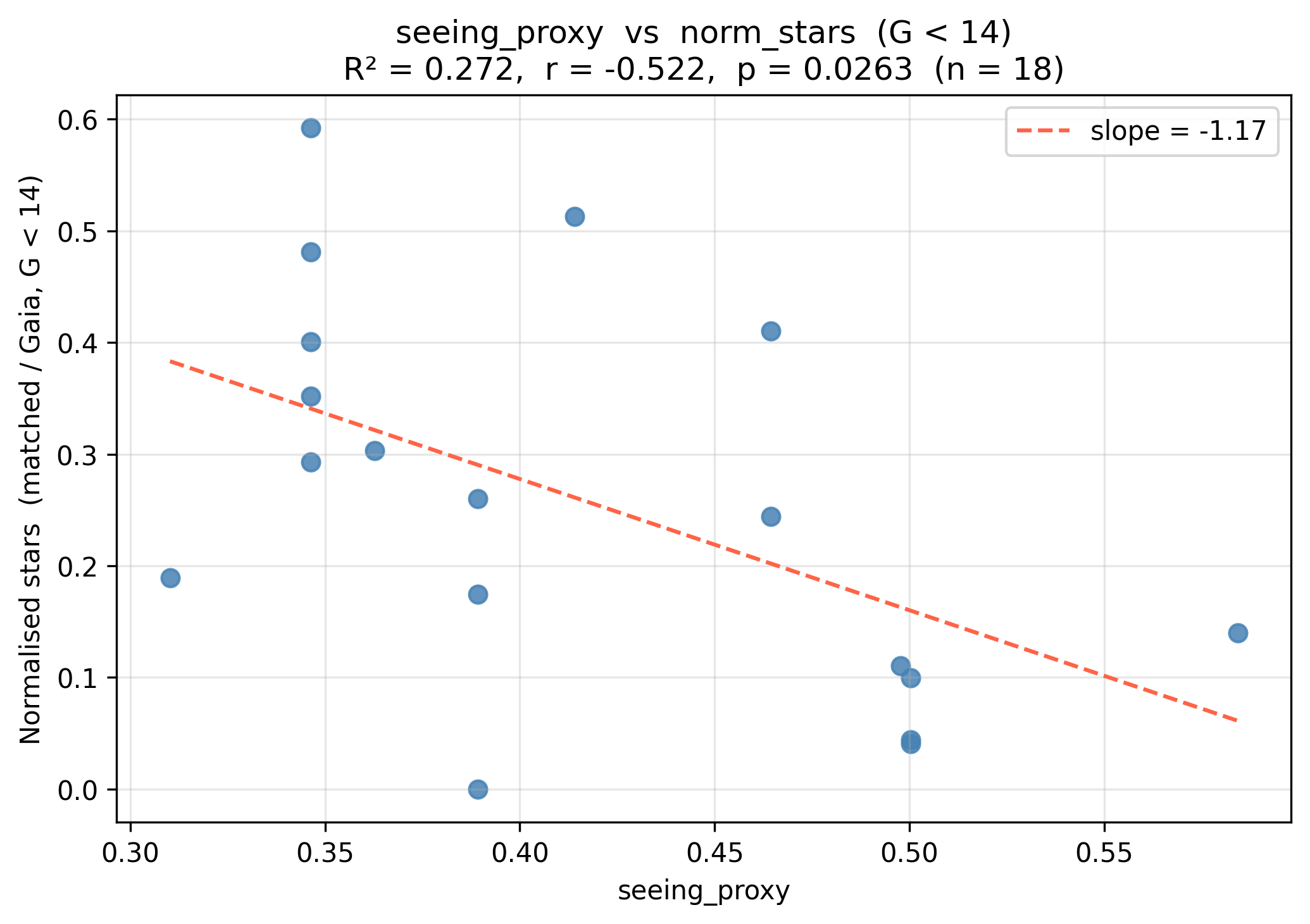
The seeing proxy produced a correlation whose sign and magnitude matched physical expectations, r = -0.522, R^2 = 0.272, p = 0.026, and slope = -1.17, the relationship has a moderate positive correlation. Higher seeing values (worse seeing conditions) were matched to lower detection ratios, this is consistent with the idea that atmospheric turbulence spreads stellar light across more pixels, reducing peak signal-to-noise and increasing blending in crowded fields. Although there still is some scatter, especially at lower seeing proxy values, the negative trend indicates that this relationship is identified as consistent with atmospheric turbulence being a factor that affects detection performance, As observed in Figure 11.

Wind speed at 10 m

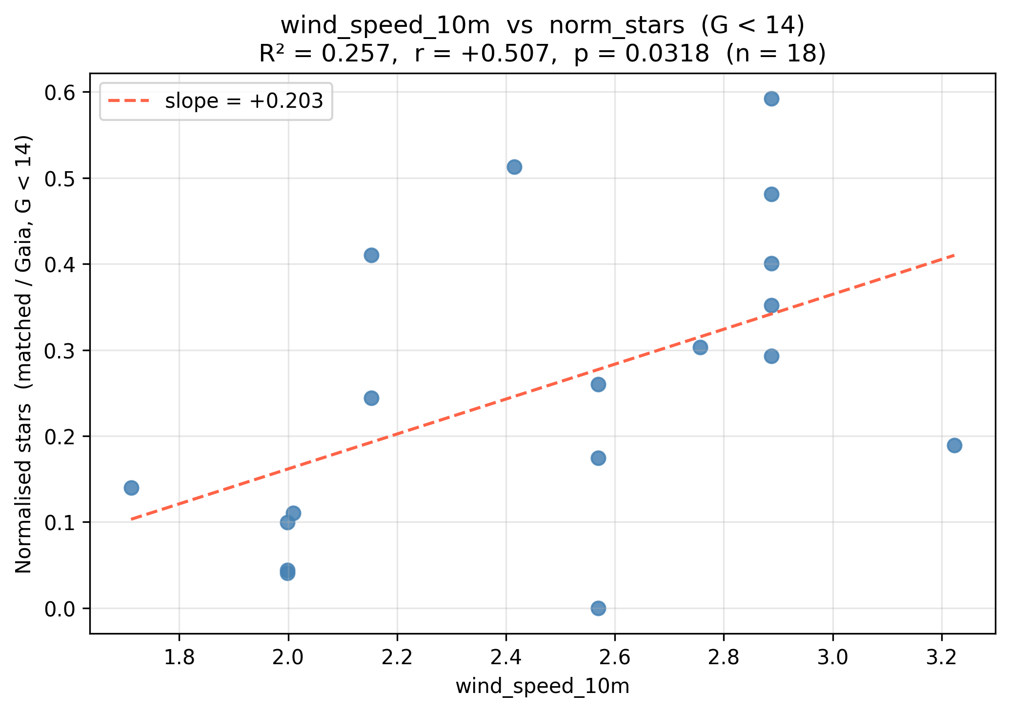
Wind speed on the other hand showed a positive correlation with efficiency, with the r = +0.507, R^2 = 0.257, p = 0.032, slope = +0.203. The positive direction is unexpected, because generally wind is interpreted as a turbulent factor that should degrade the seeing and reduce detection. It is possible that in this dataset, windier nights coincided with drier or less hazy air, some effects that would improve the transparency. Furthermore the relationship could be confounded, where wind conditions correlate with observation timing or target selection rather than directly causing a change in detection. In conclusion, the sign reversal is notable and consistent with the general patterns where confounding variables affect datasets, This sign is opposite to physical reality; the result is inconclusive and does not represent an atmospheric correlation, given the small sample size in question, with a similar field-density confounding to that described in the low-cloud-cover analysis applying here. As observed in Figure 12.

Total cloud cover

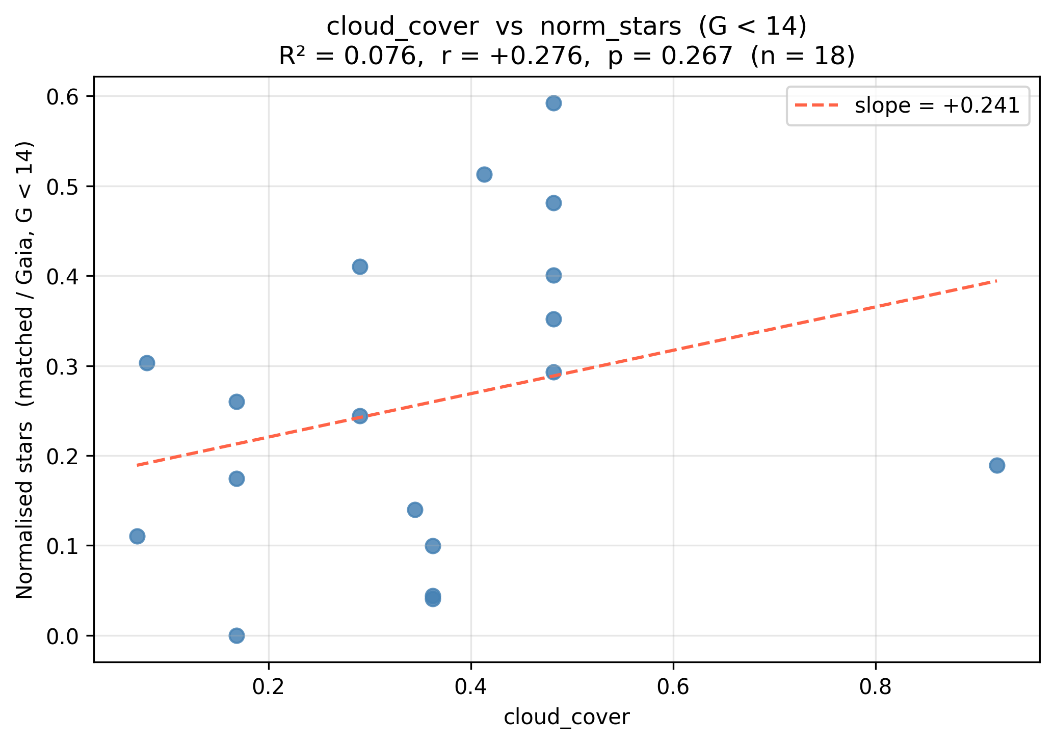
The total cloud cover has shown a weak positive correlation with r = +0.276, R^2 = 0.076, p = 0.267, slope = +0.241. The direction of the trend line is opposite, and does not match physical expectations, the expected strong negative correlation does not appear within the 18 available observations As with the other wrong-signed variables, this result is treated as inconclusive rather than as an atmospheric correlation, subject to the same field-density confounding., as observed in Figure 13.

Scatter, confounding, and limitations

Within each of the images there is a lot of scatter visible in every plot. That suggests that not any atmospheric condition, on its own, has the ability to explain the observed variation, a lot of this variance is due to different factors other than variables being plotted. These discrepancies are most likely caused by different confounding factors that vary from each observation. The 18 observations target multiple targets, dates, stacking depths, and elevation angles, and these factors are not independent of the atmospheric conditions. A night with high cloud cover could also be a night on which I pointed at a field with higher star density and stacked more frames, or even observed closer to the horizons. The anomalously strong, wrong-sign result for low cloud cover is the clearest example of this: an R^2 of 0.56 at p = 0.0003 is statistically striking, but a physically impossible positive sign means the correlation is tracking something else, not cloud-induced attenuation. Finally a limitation includes the 0.25 spatial and hourly temporal resolution of ERA5, which is low compared to how the transparency actually would vary. This mismatch deserves emphasis: each ERA5 grid cell spans 0.25°, roughly 25–31 km at mid-latitudes, so the extracted variables represent an area average over hundreds of square kilometres rather than the conditions directly above the telescope, and the hourly time step is coarse relative to exposures taken over minutes. Localised effects such as patchy low cloud, ground fog, or heat-island turbulence can therefore differ substantially from the grid-cell mean and add unquantified noise to every atmospheric predictor. ERA5 nonetheless remains a reasonable first-order proxy, as it is globally consistent, freely available, and validated against surface observations, and it is the only practical source of co-temporal conditions for archival amateur observations that lack on-site instrumentation. Even so, this representativeness error would attenuate any true correlation and is a further reason the atmospheric analysis is treated as exploratory. Next the linear assumptions in the regressions cannot capture the effects of threshold on the images. To determine whether a linear model was suitable, given that the detection ratio is bounded between 0 and 1, the residuals of each regression were inspected and the regressions were run again using a logit transform of the ratio. The residual plots showed neither an apparent curvilinear nor a funnelling pattern, and the signs of all relationships remained unchanged under transformation, indicating that the linear specification has not distorted the directionality of any relationship. While the strengths of the correlations did reduce upon transformation — for example, the seeing and wind-speed relationships, both already non-significant after Bonferroni correction, reduced further to p = 0.21 and p = 0.19 respectively — this is in line with the exploratory nature of the atmospheric investigation rather than with any non-linear form.

This pattern is characteristic of a small, heterogeneous sample in which confounding variables correlate incidentally with atmospheric conditions. A Bonferroni correction was applied to the five atmospheric variables that were tested simultaneously, giving a significance threshold of α = 0.05/5 = 0.01. Under this threshold only the low-level cloud result remains “significant” (p = 0.0003). The seeing and wind-speed correlations, where p = 0.026 and 0.032 respectively, initially seemed significant at the uncorrected level but now do not pass the test, and the total-cloud-cover and transparency proxies were never significant. Hence, the only result that survives the test is the low-cloud correlation, which is physically impossible in sign and is attributable to field-density confounding, as explained throughout the manuscript; it is therefore safe to conclude that no atmospheric correlation is physically interpretable, given the small sample size and the exploratory nature of the study. With n = 18, the minimum reliably detectable correlation is |r| ≈ 0.47 (rising to |r| ≈ 0.59 after Bonferroni correction). Furthermore, the power to detect a moderate true effect (r = 0.5) is only about 0.57, and stable correlation estimates would require at least 30 observations. Adjusted R² values, which penalise small samples, are 0.54 (low-level cloud), 0.23 (seeing), 0.21 (wind speed), and 0.02 (total cloud and transparency). Bootstrap 95% confidence intervals on Pearson r (10,000 resamples) were computed for each correlation: low-level cloud [+0.545, +0.898]; seeing [−0.784, −0.199]; wind speed [+0.152, +0.797]; total cloud [−0.034, +0.687]; transparency [−0.699, +0.038]. The total-cloud and transparency intervals include zero, confirming that these correlations are not robust at such a sample size, restating the exploratory nature of the study. The methodology is sound, but a larger dataset, homogeneous target selection, or multivariate regression with confounder controls would be required to isolate genuine atmospheric dependencies with high confidence. The current results should therefore be interpreted as an exploratory analysis, and not as proof that the pipeline can detect atmospheric signals. None of the atmospheric variables produced a correlation that was both statistically robust, surviving the correction, and physically interpretable in its sign. The value of this section lies in demonstrating the framework of the analysis and in exposing the confounding factors that must be controlled in future work, rather than in quantifying how atmospheric conditions govern detection performance.

Conclusion

The analysis demonstrated that the normalised star ratio is a well defined and comparable metric that the pipeline produces reasonable detection behavior across the 18 image files. Three out of the five relationships produce sign reversals relative to physical expectation, and the strongest correlation in the dataset (low-level cloud cover, R^2 = 0.56) is among them. This pattern is a characteristic of the small and heterogenous sample in which confounding factors correlate with atmospheric conditions. The core validity of the pipeline is supported by the photometric analysis, whose fitted slopes are statistically consistent with the theoretical magnitude–flux relationship. The atmospheric analysis, on the other hand, is exploratory: after the correction for multiple comparisons, no atmospheric correlation was both statistically robust and physically interpretable, and the strongest apparent correlation is attributable to field-density confounding. Isolating genuine atmospheric dependencies would require a larger dataset, homogeneous or repeated target selection to break the coupling between target and weather, and multivariate control of confounders such as field density, stacking depth, and target elevation.

References

1. Hubble, E. (1929). “A relation between distance and radial velocity among extra-galactic nebulae.” Proc. Natl. Acad. Sci. 15(3): 168–173. [↩]
2. LSST Collaboration. (2019). “LSST: From science drivers to reference design and anticipated data products.” Astrophys. J. 873: 111. [↩]
3. Wells, D. C., Greisen, E. W., and Harten, R. H. (1981). “FITS: A flexible image transport system.” Astron. Astrophys. Suppl. Ser. 44: 363–370. [↩]
4. Greisen, E. W. and Calabretta, M. R. (2002). “Representations of world coordinates in FITS.” Astron. Astrophys. 395: 1061–1075. [↩]
5. Howell, S. B. (2006). Handbook of CCD Astronomy (2nd ed.). Cambridge University Press. [↩]
6. Astropy Collaboration. (2013). “Astropy: A community python package for astronomy.” Astron. Astrophys. 558: A33. [↩]
7. Astropy Collaboration. (2018). “The astropy project: Building an open-science project and status of the v2.0 core package.” Astron. J. 156: 123. [↩]
8. Budávári, T. and Szalay, A. S. (2008). “Probabilistic cross-identification of astronomical sources.” Astrophys. J. 679: 301–309. [↩]
9. Gaia Collaboration, Vallenari, A., et al. (2023). “Gaia Data Release 3: Summary of the content and survey properties.” Astron. Astrophys. 674: A1. [↩]
10. Gaia Collaboration. (2016). “The Gaia mission.” Astron. Astrophys. 595: A1. [↩]
11. Gaia Collaboration. (2018). “Gaia data release 2: Summary of the contents and survey properties.” Astron. Astrophys. 616: A1. [↩]
12. Lindegren, L., Hernández, J., Bombrun, A., Klioner, S., Bastian, U., Ramos-Lerate, M., de Torres, A., Steidelüller, H., Stephenson, C., Hobbs, D., Lammers, U., Biermann, M., Geyer, R., Hilger, T., Michalik, D., Stampa, U., McMillan, P. J., Castañeda, J., Clotet, M., Comoretto, G., Davidson, M., Fabricius, C., Gracia, G., Hambly, N. C., Hutton, A., Mora, A., Portell, J., van Leeuwen, F., Abbas, U., Abreu, A., Altmann, M., Andrei, A., Anglada, E., Balaguer-Núñez, L., Barache, C., Becciani, U., Bertone, S., Bianchi, L., Bouquillon, S., Bourda, G., Brüsemeister, T., Bucciarelli, B., Busonero, D., Buzzi, R., Cancelliere, R., Carlucci, T., Charlot, P., Cheek, N., Crosta, M., Crowley, C., de Bruijne, J., de Felice, F., Drimmel, R., Esquej, P., Fienga, A., Fraile, E., Gai, M., Garralda, N., González-Vidal, J. J., Guerra, R., Hauser, M., Hofmann, W., Holl, B., Jordan, S., Lattanzi, M. G., Lenhardt, H., Liao, S., Licata, E., Lister, T., Löffler, W., Marchant, J., Martin-Fleitas, J., Messineo, R., Mignard, F., Morbidelli, R., Poggio, E., Riva, A., Rowell, N., Salguero, E., Sarasso, M., Sciacca, E., Siddiqui, H., Smart, R. L., Spagna, A., Steele, I., Taris, F., Torra, J., van Elteren, A., van Reeven, W., and Vecchiato, A. (2018). “Gaia data release 2: The astrometric solution.” Astron. Astrophys. 616: A2. [↩]
13. Bertin, E. and Arnouts, S. (1996). “SExtractor: Software for source extraction.” Astron. Astrophys. Suppl. Ser. 117: 393–404. [↩]
14. Stetson, P. B. (1987). “DAOPHOT: A computer program for crowded-field stellar photometry.” Publ. Astron. Soc. Pac. 99: 191–222. [↩]
15. Racine, R. (1996). “The telescope point spread function.” Publ. Astron. Soc. Pac. 108: 699–705. [↩]
16. Stetson, P. B. (1992). “Further progress in CCD photometry.” In Astronomical Data Analysis Software and Systems I, 25:297. [↩]
17. Mighell, K. J. (1999). “Algorithms for CCD stellar photometry.” In Astronomical Data Analysis Software and Systems VIII, 172:317. [↩]
18. Howell, S. B. (2006). “Photometry and astrometry.” In Handbook of CCD Astronomy. Cambridge University Press. [↩]
19. Cinzano, P., Falchi, F., and Elvidge, C. D. (2001). “The first world atlas of the artificial night sky brightness.” Mon. Not. R. Astron. Soc. 328: 689–707. [↩]
20. Falchi, F., Cinzano, P., Duriscoe, D., Kyba, C. C. M., Elvidge, C. D., Baugh, K., Portnov, B. A., Rybnikova, N. A., and Furgoni, R. (2016). “The new world atlas of artificial night sky brightness.” Sci. Adv. 2: e1600377. [↩]
21. Kyba, C. C. M., Kuester, T., Sánchez de Miguel, A., Baugh, K., Jechow, A., Hölker, F., Bennie, J., Elvidge, C. D., Gaston, K. J., and Guanter, L. (2017). “Artificially lit surface of earth at night increasing in radiance and extent.” Sci. Adv. 3: e1701528. [↩]
22. Garstang, R. H. (1989). “Night-sky brightness at observatories and sites.” Publ. Astron. Soc. Pac. 101: 306–329. [↩] [↩]
23. Duriscoe, D. M. (2013). “Measuring anthropogenic sky glow using a natural sky brightness model.” Publ. Astron. Soc. Pac. 125: 1370–1382. [↩] [↩]
24. Kyba, C. C. M., Tong, K. P., Bennie, J., Birriel, I., Birriel, J. J., Cool, A., Danielsen, A., Davies, T. W., den Outer, P. N., Edwards, W., Ehlert, R., Falchi, F., Fischer, J., Giacomelli, A., Giubbilini, F., Haaima, M., Hesse, C., Heygster, G., Hölker, F., Inger, R., Jensen, L. J., Kuechly, H. U., Kuehn, J., Langill, P., Lolkema, D. E., Nagy, M., Nievas, M., Ochi, N., Popow, E., Posch, T., Puschnig, J., Ruhtz, T., Schmidt, W., Schwarz, R., Schwope, A., Spoelstra, H., Tekatch, A., Trueblood, M., Walker, C. E., Weber, M., Welch, D. L., Zamorano, J., and Gaston, K. J. (2015). “Worldwide variations in artificial skyglow.” Sci. Rep. 5: 8409. [↩]
25. Lang, D., Hogg, D. W., Mierle, K., Blanton, M., and Roweis, S. (2010). “Astrometry.net: Blind astrometric calibration of arbitrary astronomical images.” Astron. J. 139: 1782–1800. [↩]
26. ZWO Optical. (2023). Seestar S50 Smart Telescope Technical Documentation. [↩]
27. Copernicus Climate Change Service (C3S). (2017). ERA5: Fifth generation of ECMWF atmospheric reanalyses of the global climate. Copernicus Climate Change Service Climate Data Store (CDS). https://cds.climate.copernicus.eu/ [↩]
28. Hersbach, H., Bell, B., Berrisford, P., Hirahara, S., Horányi, A., Muñoz-Sabater, J., Nicolas, J., Peubey, C., Radu, R., Schepers, D., Simmons, A., Soci, C., Abdalla, S., Abellan, X., Balsamo, G., Bechtold, P., Biavati, G., Bidlot, J., Bonavita, M., De Chiara, G., Dahlgren, P., Dee, D., Diamantakis, M., Dragani, R., Flemming, J., Forbes, R., Fuentes, M., Geer, A., Haimberger, L., Healy, S., Hogan, R. J., Hólm, E., Janisková, M., Keeley, S., Laloyaux, P., Lopez, P., Lupu, C., Radnoti, G., de Rosnay, P., Rozum, I., Vamborg, F., Villaume, S., and Thépaut, J. (2020). “The ERA5 global reanalysis.” Q. J. R. Meteorol. Soc. 146: 1999–2049. [↩]
29. Hänel, A., et al. (2018). “Measuring night sky brightness: Methods and challenges.” J. Quant. Spectrosc. Radiat. Transfer 205: 278–290. [↩]